Introduction
The R add-on package gmkin provides a browser based graphical interface for performing kinetic evaluations of degradation data using the mkin package. While the use of gmkin should be largely self-explanatory, this manual may serve as a functionality overview and reference.
For system requirements and installation instructions, please refer to the gmkin homepage.
Starting gmkin
As gmkin is an R package, you need to start R and load the gmkin package before you can run gmkin. The latter can be achieved by entering the command
into the R console. This will also load the packages that gmkin depends on, most notably gWidgetsWWW2 and mkin. Loading the package only has to be done once after you have started R.
Before you start gmkin, you should make sure that R is using the working directory that you would like to keep your gmkin project file(s) in. If you use the standard R GUI application on windows, you can change the working directory from the File menu (‘File’ -> ‘Change dir…’).
Once you are sure that the working directory is what you want it to be, gmkin can be started by entering the R command
gmkin()This will cause the default browser to start up or, if it is already running, to pop up and open a new tab for displaying the gmkin user interface.
In the R console, you should see a message that the httpd help server is started, if it wasn’t already started before.
In the browser, you should see something like the screenshot below.
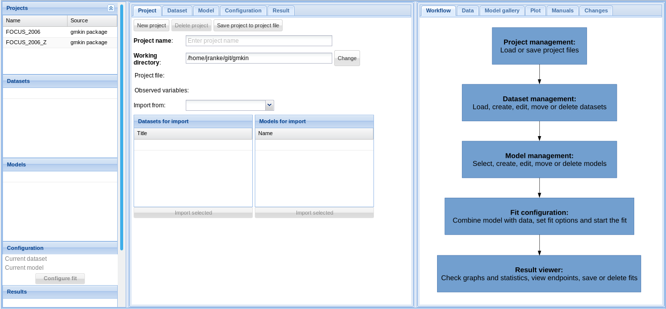
Screenshot of the newly started gmkin GUI
The statusbar at the bottom of the gmkin window shows, among others, the working directory that gmkin uses.
If the browser only shows “Loading ExtJS…” and nothing else happens for about 10 to 15 seconds, please enter the gmkin() command again in the R console. If this still does not bring up the gmkin GUI, please close the browser and try again.
Three column layout
Since version 0.6.1, gmkin adheres to a three column layout. To the left, there are explorer areas for the available projects, datasets, kinetic models and the completed fits.
In the central, tabbed area, the projects, datasets, models and fits are defined. The area to the right is mainly for showing information intended to support the user, and results. However, it also contains a tab ‘Data’ for editing kinetic data.
Project file management
At startup, the project explorer to the left shows the two project workspaces ‘FOCUS_2006’ and ‘FOCUS_2006_Z’ delivered with the package. The project manangement area in the center gives the possibility to save these projects under a new name, or to start a new, empty project.
A gmkin project workspace contains datasets, kinetic models for fitting, and so-called fits, i.e. the results of fitting models to data. The project area also shows the current working directory, where project workspace files are saved using the file extension .gmkinws.
Once a project has been saved by the user, the project explorer to the left will show it in the project list.

Screenshot of saving a new project
The current state of a project should repeatedly be saved during the work in order to avoid loosing data. This can be achieved by selecting the ‘Project’ tab in the center and pressing the ‘Save project to project file’ button. More conveniently, the keyboard shortcut Shift-F12 (was Ctrl-X in gmkin < 0.6.6) can be used to save the current status of the project.
In the project file management area, datasets and models can be imported from one of the projects in the project list, once it has been selected in the droplist labelled ‘Import from:’.
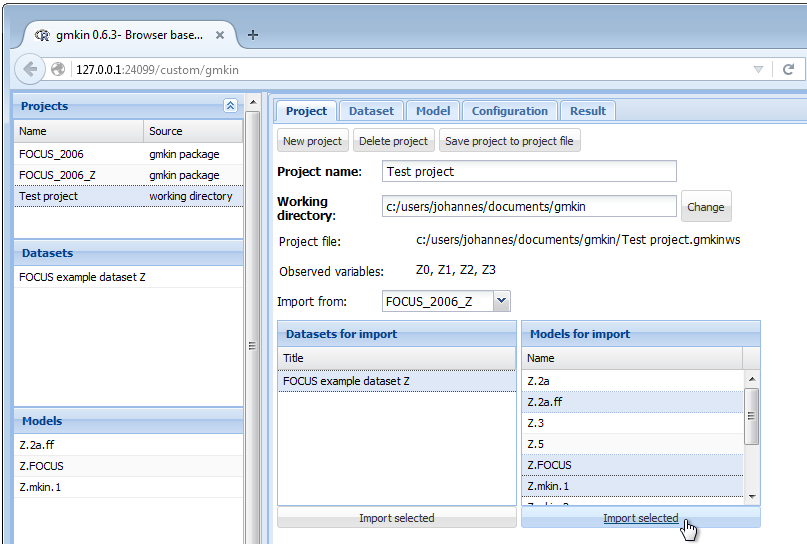
Screenshot of importing datasets and models
Once the project has been set up, you may want to minimize the project explorer, especially if you are limited in vertical screen space.
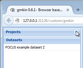
Screenshot of minimized project explorer
Dataset editor
When you select one of the datasets in the dataset explorer to the left, some summary information about the dataset is shown in the center, and the data itself is loaded into the data editor to the right.
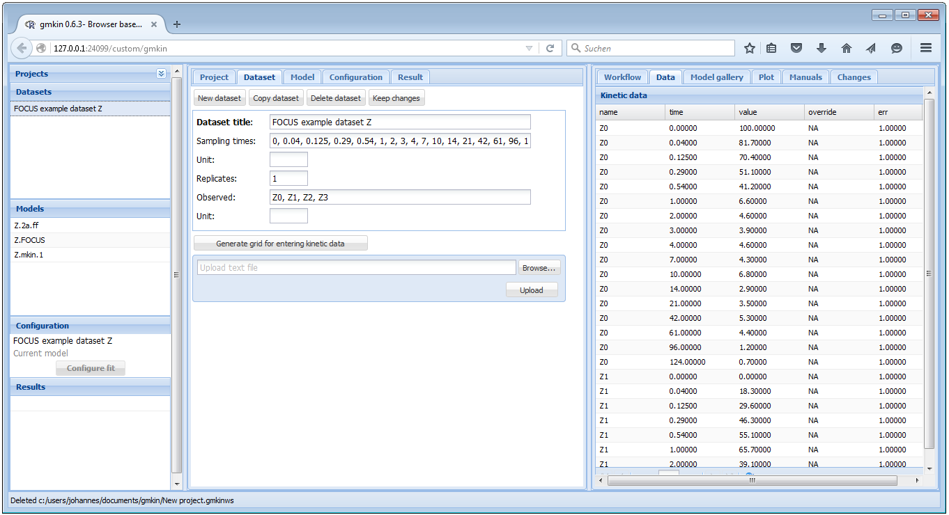
Screenshot of the GUI after loading a dataset
When you have added information about the units, or edited the data to the right, you should hit the button ‘Keep changes’. This will add a new entry in the dataset explorer.
In the dataset editor to the right, you can override original data (for example in order to follow FOCUS recommendations for time zero samples or values below the limit of detection) by entering numbers in the override column.
When saving a dataset, the sampling times, the number of replicates and the list of observed variables will be computed from the current data in the data editor.
However, entering data in these fields is a prerequisite for entering a new dataset directly in the dataset editor.
Entering data directly
For entering new data manually, there are two possibilities. You can either change the Dataset title of the current dataset and edit the data in the Data editor to the right. Or, if the new data should have a different structure, e.g. different sampling times, observed variables and replicates, click on “New dataset”, edit the dataset title, sampling times, number of replicates and the list of observed variables, and press the button ‘Generate grid for entering kinetic data’, in order to prepare the Data editor to the right.
For sampling times and short names of the relevant compounds, a comma separated list must be entered, with a space after each comma. An example of filling out the respective fields is shown below.
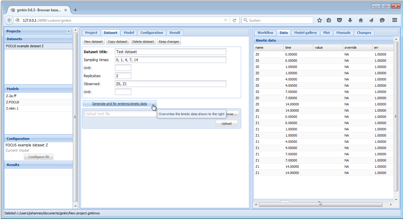
Screenshot of generating a data grid
After that, the actual measurements can be entered into the Data editor to the right, in the column ‘value’.
If everything is OK, press “Keep changes” to save the dataset in the current workspace. Note that you need to save the project file (see above) in order to be able to use the dataset that you created in a future gmkin session.
Importing data from text files
In case you want to work with a larger dataset that is already available as a computer file e.g. in a spreadsheet application, you can export these data as a tab separated or comma separated text file and import it using the “Browse” and “Upload” buttons in the dataset editor.
As an example, we can create a text file from one of the datasets shipped with the mkin package using the following R command:
write.table(schaefer07_complex_case, sep = ",", dec = ".",
            row.names = FALSE, quote = FALSE,
            file = "schaefer07.csv")
This produces a text file with comma separated values in the current working directory of R.
Loading this text file into gmkin using the “Browse” and “Upload” buttons
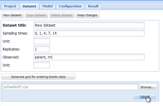
Screenshot of the browse and upload dialogue
results in an an import configuration area showing the top lines of the imported file, and giving the possibility to chose the import options matching the file format.
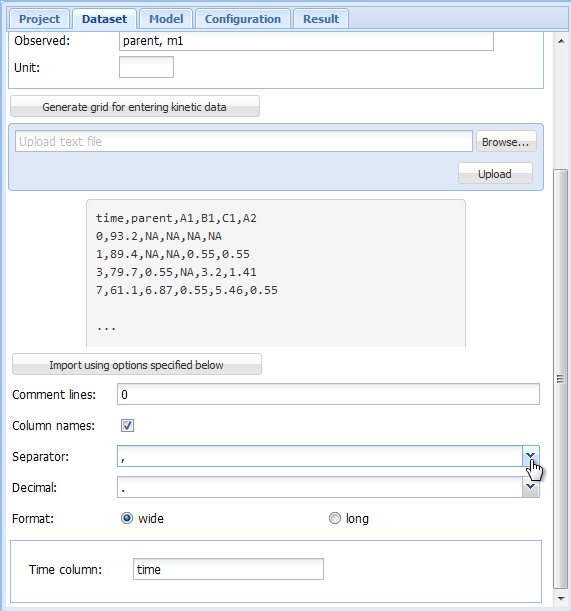
Screenshot of the import configuration area
In the import configuration area, the following options can be specified. In the field “Comment lines”, the number of lines in the beginning of the file that should be ignored can be specified.
The checkbox on the next line should be checked if the first line of the file contains the column names, i.e. the names of the observed variables when the data are in wide format.
As “Separator”, whitespace, semicolon or comma can be chosen. If whitespace is selected, files in which the values are separated by a fixed or varying number of whitespace characters should be read in correctly. As the tabulator counts as a whitespace character, this is also the option to choose for tabulator separated values.
As the “Decimal” separator, comma “,” or period “.” can be selected.
In the next line, it can be specified if the data are in wide or in long format. If in wide format, the only option left to specify is the title of the column containing the sampling times. If the data is in long format, the column headings specifying the columns containing the observed variables (default is “name”), the sampling times (default is “time”), the observed values (default is “value”) and, if present in the data, the relative errors (default is “err”) can be adapted. The default settings appearing if the long format is selected are shown below.
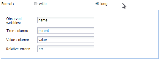
Screenshot of the default variable names for data in long format
In our example we have data in the wide format, and after adapting the “Separator” to a comma, we can press the button “Import using options specified below”, and the data should be imported. If successful, the dataset editor should show the sampling times and the names of the observed variables, and the Data editor should show the imported data in a grid for further editing or specifying overrides.
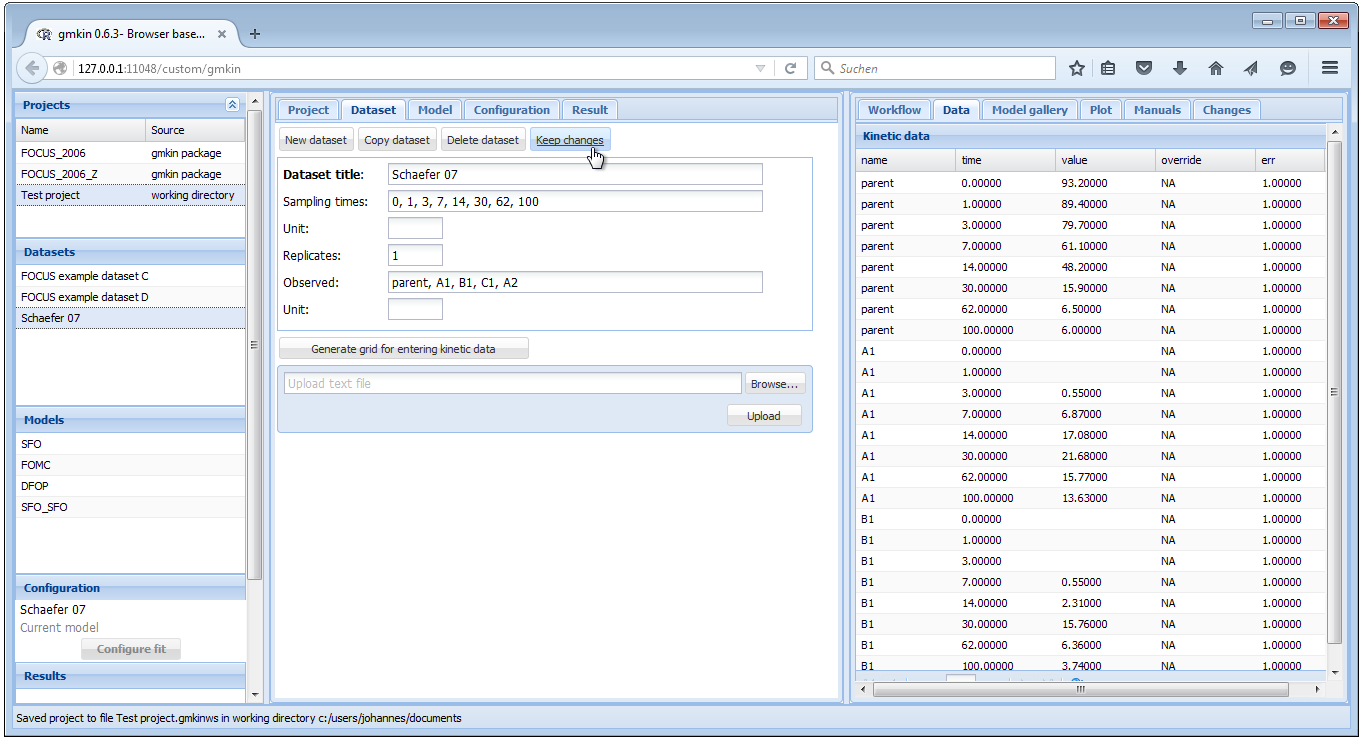
Screenshot of a successful upload
After adapting the dataset title and possibly the units, press “Keep changes” to save the dataset in the current workspace. Again, you need to save the project file in order to be able to use the dataset that you created in a future gmkin session.
Model editor
The following screenshot shows the model editor for the model ‘Z.2a.ff’ from the project workspace ‘FOCUS_2006_Z’ provided with the gmkin package.
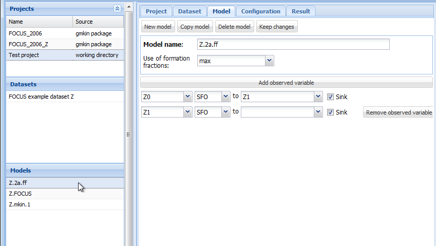
Screenshot of the model editor
In the first line the name of the model can be edited. You can also specify “min” or “max” for minimum or maximum use of formation fractions. Maximum use of formation fractions means that the differential equations in the degradation model are formulated using formation fractions. When you specify “min”, then formation fractions are only used for the parent compound when you use the FOMC, DFOP or the HS model for it.
Pressing “Add observed variable” adds a line in the array of state variable specifications below. The observed variables to be added are usually transformation products (usually termed metabolites), but can also be the parent compound in a different compartment (e.g. “parent_sediment”).
Only observed variable names that occur in previously defined datasets or models can be selected. For any observed variable other than the first one, only the SFO or the SFORB model can be selected. For each observed variables, a comma separated list of target variables can be specified. In addition, a pathway to the sink compartment can be selected. If too many observed variables have been added, complete lines can be removed from the model definition by pressing the button “Remove observed variable”.
If the model definition is supposedly correct, press “Keep changes” to make it possible to select it for fitting in the listing of models to the left.
Configuring the fit
If a dataset and a kinetic model are selected, the button “Configure fit” below in the Explorer window “Configuration” becomes active. Pressing it opens the “Configuration” area in the center and loads the dataset into the Data editor to the right, for viewing only.
After pressing the button ‘Plot unoptimised’, the data and the kinetic model with default starting parameters are plotted in the ‘Plot’ area to the right.
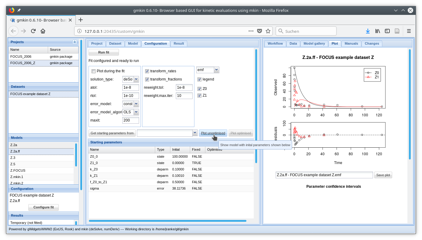
Screenshot of the fit configuration area
Fit options
The most important fit options of the mkinfit function can be set via the controls in the fit configuration area shown above. If the “plot” checkbox is checked (and on Windows, the R GUI is used for running gmkin), an R graphics device started via the R console shows the fitting progress, i.e. the change of the model solution together with the data during the optimisation.
The “solution_type” can either be “auto”, which means that the most effective solution method is chosen for the model, in the order of “analytical” (for parent only degradation data), “eigen” (for differential equation models with only linear terms, i.e. without FOMC, DFOP or HS submodels) or “deSolve”, which can handle all model definitions generated by the mkin package. If a compiler (gcc, on Windows install the ‘Rtools’ software package), then the “deSolve” solution method is alway chosen when there are more than one variables in the model.
The parameters “atol” and “rtol” are only effective if the solution type is “deSolve”. They control the precision of the iterative numerical solution of the differential equation model.
The checkboxes “transform_rates” and “transform_fractions” control if the parameters are fitted as defined in the model, or if they are internally transformed during the fitting process in order to improve the estimation of standard errors and confidence intervals which are based on a linear approximation at the optimum found by the fitting algorithm.
If fitting with transformed fractions leads to a suboptimal fit, doing a first run without transforming fractions may help. A final run using the optimised parameters from the previous run as starting values (see comment on “Get initials from” above) can then be performed with transformed fractions.
If the “error_model” option is set to “obs” or “tc”, then a suitable “error_model_algorithm” has to be selected. The recommended algorithm for these error model is “d_3”, which is the one selected by “mkin” for there error models. Please refer to the mkinfit documentation for more details. IRLS fitting can be configured using the options “reweight.tol” and “reweight.max.iter”.
The maximum number of iterations for the optimisation can be adapted using the “maxit” field.
Plot options
In the right part of the fit configuration area, the file format can be chosen, the legend can be turned off, and the observed variables for which the data and the model fit should be plotted can be selected as shown below.
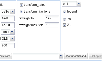
plot options
On systems running the Windows operating system, the enhanced metafile (emf) format can be additionally chosen. Changing the file format for plotting will also change the extension of the proposed filename for saving the plot.
Parameters
Below the fit control area, a table with the Starting parameter list is displayed. While name and type of the parameters should not be edited, their initial values can be edited by clicking on a row. Also, it can be specified if the parameters should be fixed in the optimisation process.
If the initial values for the parameters were changed, the resulting model solution can be visually checked by pressing the button “Plot unoptimised”. This will update the plot of the model and the data using the specified initial parameter values.
If a similar model with a partially overlapping model definition has already be fitted, initial values for parameters with the same name in both models can also be retrieved from previous fits by selecting the fit and pressing the button “Get starting parameters from”. This facilitates stepwise fitting of more complex degradation pathways.
After the model has been successfully fitted by pressing the “Run fit” button, the optimised parameter values are added to the parameter table.
Fitting the model
In many cases the starting parameters and the fit options do not need to be modified and the model fitting process can simply be started by pressing the “Run fit” button. In the R console, the progressive reduction in the model cost can be monitored and will be displayed in the following way:
> Ordinary least squares optimisation
Sum of squared residuals at call 1: 2388.077
Sum of squared residuals at call 3: 2388.077
Sum of squared residuals at call 4: 247.1962
Sum of squared residuals at call 7: 200.6791
Sum of squared residuals at call 10: 197.7231
Sum of squared residuals at call 11: 197.0872
Sum of squared residuals at call 14: 196.535
Sum of squared residuals at call 15: 196.535
Sum of squared residuals at call 16: 196.535
Sum of squared residuals at call 17: 196.5334
Sum of squared residuals at call 20: 196.5334
Sum of squared residuals at call 25: 196.5334
Negative log-likelihood at call 31: 26.64668
Optimisation successfully terminated.
If plotting of the fitting progress was selected, a new separate graphics window should either pop up, or a graphics window previously started for this purpose will be reused.
If your screen size allows for it, you can arrange the R plotting window and the R console in a way that you can see everything at the same time:
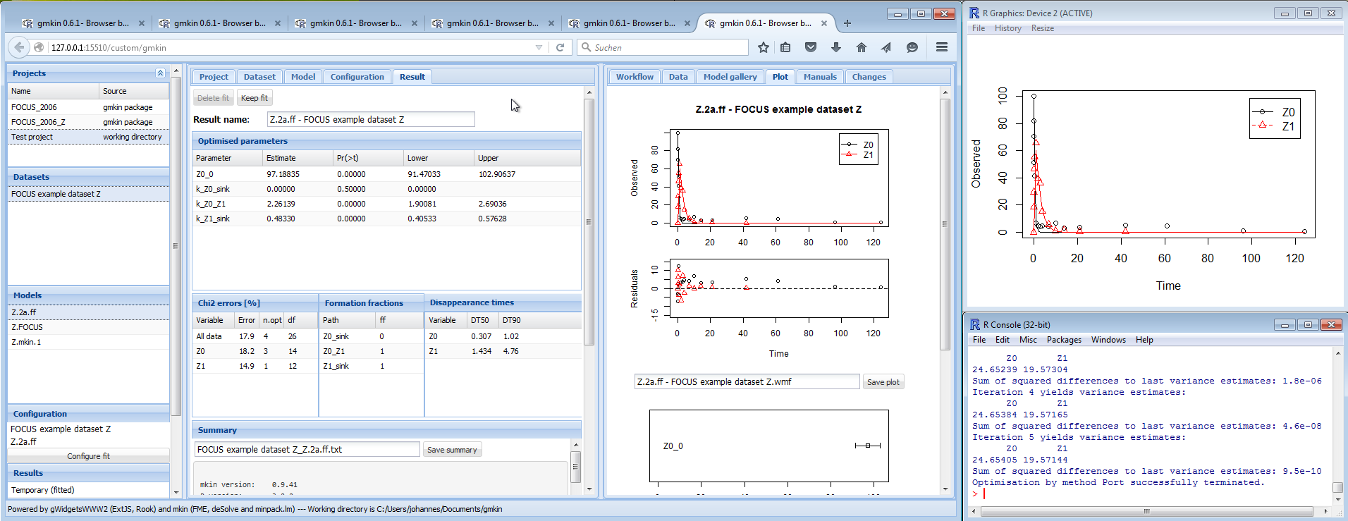
Screenshot of arrangement of plot window and console
Results and summary
Once a fit has successfully been completed, the most important results are shown in several tables in the “Result” area as shown below.
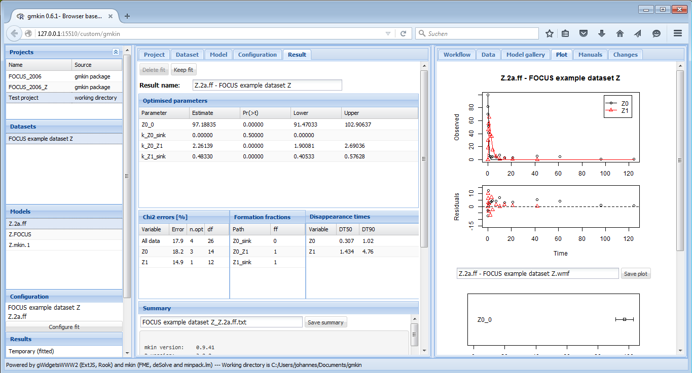
Screenshot of the results
The detailed summary can be accessed below these tables.
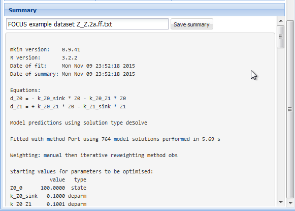
Screenshot of the summary
The complete summary can be saved into a text file by specifying a suitable file name and pressing the button “Save summary”.
Confidence interval plots
Whenever a new fit has been configured or a run of a fit has been completed, the plotting area is updated with the abovementioned plot of the data and the current model solution.
In addition, a confidence interval plot is shown below this conventional plot. In case a fit has been run and confidence intervals were successfully calculated for the fit (i.e. if the model was not overparameterised and no other problems occurred), the confidence intervals are graphically displayed as bars as shown below.
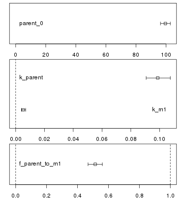
confidence
Howtos
The following sections show step by step descriptions of how to perform certain tasks using gmkin. In principle, this should not be necessary as the GUI was designed to be largely self-explanatory. Nevertheless it may help a beginner to understand how to use gmkin. At the same time, the gmkin author uses them as test cases to make sure that the most important functionality is not broken before releasing a new version.
1. Use a model and a dataset from a built-in workspace
- Start gmkin
- In the project explorer, select the project ‘FOCUS_2006’
- In the dataset explorer, select ‘FOCUS example dataset C’
- In the model explorer, select ‘SFO’
- In the configuration display, press ‘Configure fit’
- In the configuration editor in the center, press ‘Run fit’
- In the pop-up window that appears, press ‘Yes’
- In the result viewer in the center, press ‘Keep fit’
- Switch to the Project editor in the center
- Check that the working directory is OK for writing a test project
- If not, enter a suitable path (e.g. “~” which will be resolved to your home directory) and press ‘Change’
- In the project explorer, enter the project name ‘Howto test 1’
- Press ‘Save project to project file’
2. Enter a simple dataset and evaluate it using a model from the gallery
- Start gmkin
- In the project explorer, enter the project name ‘Howto test 2’
- Press ‘Save project to project file’
- Select the dataset editor in the center
- Enter dataset title ‘Data howto 2’
- Enter sampling times ‘0, 1, 3, 7, 14’
- Enter replicates ‘1’
- Enter observed variable ‘parent, A1’
- Press ‘Generate grid for entering kinetic data’
- In the value column of the dataset editor, enter values ‘100’, ‘30’, ‘10’, ‘5’, ‘3’, ’’ (nothing), ‘3’, ‘8’, ‘7’, ‘5’
- Press ‘Keep changes’
- Select the ‘Model gallery’ to the right
- From the model gallery, press ‘FOMC, one met’ below the corresponding model scheme
- In the dataset explorer, select ‘Data howto 2’
- In the model explorer, select ‘FOMC, one met’
- In the configuration display, press ‘Configure fit’
- In the configuration editor in the center, press ‘Run fit’
- In the pop-up window that appears, press ‘Yes’
- In the result viewer in the center, press ‘Keep fit’
- Switch to the Project editor in the center
- Press ‘Save project to project file’
3. Load a tab separated input file in wide format and evaluate using a newly created model
- Start gmkin
- In the project explorer, enter the project name ‘Howto test 3’
- Press ‘Save project to project file’
- Select the dataset editor in the center
- In the data upload widget, press ‘Browse’
- Select the file ‘testdata/d_synth_DFOP_lin_c.txt’ from gmkin installation
- Press ‘Upload’
- Press ‘Import using options specified below’
- Enter dataset title ‘DFOP lin c’
- Press ‘Keep changes’
- Select the model editor in the center
- Press ‘New model’
- Enter ‘DFOP lin’ as the model name
- Select ‘max’ in the dropbox ‘Use of formation fractions’
- Press ‘Add observed variable’ three times
- In the line where ‘parent’ is selected, in the dropbox to the right change ‘SFO’ to ‘DFOP’
- In the line where ‘parent’ is selected, after the word ‘to’, select ‘M1’
- Click outside the dropbox
- In the line where ‘M1’ is selected, in the dropbox after the word ‘to’, select ‘M2’
- Click outside the dropbox
- Press ‘Keep changes’
- In the dataset explorer, select ‘DFOP lin c’
- In the model explorer, select ‘DFOP lin’
- In the configuration display, press ‘Configure fit’
- In the configuration editor in the center, press ‘Run fit’
- In the pop-up window that appears, press ‘Yes’
- In the result viewer in the center, press ‘Keep fit’
- Switch to the Project editor in the center
- Press ‘Save project to project file’