Example evaluations of the dimethenamid data from 2018
Johannes Ranke
Last change 4 August 2021, built on 04 Aug 2021
Source:vignettes/web_only/dimethenamid_2018.rmd
dimethenamid_2018.rmdWissenschaftlicher Berater, Kronacher Str. 12, 79639 Grenzach-Wyhlen, Germany
Privatdozent at the University of Bremen
Introduction
During the preparation of the journal article on nonlinear mixed-effects models in degradation kinetics (submitted) and the analysis of the dimethenamid degradation data analysed therein, a need for a more detailed analysis using not only nlme and saemix, but also nlmixr for fitting the mixed-effects models was identified.
This vignette is an attempt to satisfy this need.
Data
Residue data forming the basis for the endpoints derived in the conclusion on the peer review of the pesticide risk assessment of dimethenamid-P published by the European Food Safety Authority (EFSA) in 2018 (EFSA 2018) were transcribed from the risk assessment report (Rapporteur Member State Germany, Co-Rapporteur Member State Bulgaria 2018) which can be downloaded from the EFSA register of questions.
The data are available in the mkin package. The following code (hidden by default, please use the button to the right to show it) treats the data available for the racemic mixture dimethenamid (DMTA) and its enantiomer dimethenamid-P (DMTAP) in the same way, as no difference between their degradation behaviour was identified in the EU risk assessment. The observation times of each dataset are multiplied with the corresponding normalisation factor also available in the dataset, in order to make it possible to describe all datasets with a single set of parameters.
Also, datasets observed in the same soil are merged, resulting in dimethenamid (DMTA) data from six soils.
library(mkin)
dmta_ds <- lapply(1:8, function(i) {
  ds_i <- dimethenamid_2018$ds[[i]]$data
  ds_i[ds_i$name == "DMTAP", "name"] <-  "DMTA"
  ds_i$time <- ds_i$time * dimethenamid_2018$f_time_norm[i]
  ds_i
})
names(dmta_ds) <- sapply(dimethenamid_2018$ds, function(ds) ds$title)
dmta_ds[["Borstel"]] <- rbind(dmta_ds[["Borstel 1"]], dmta_ds[["Borstel 2"]])
dmta_ds[["Borstel 1"]] <- NULL
dmta_ds[["Borstel 2"]] <- NULL
dmta_ds[["Elliot"]] <- rbind(dmta_ds[["Elliot 1"]], dmta_ds[["Elliot 2"]])
dmta_ds[["Elliot 1"]] <- NULL
dmta_ds[["Elliot 2"]] <- NULL
Parent degradation
We evaluate the observed degradation of the parent compound using simple exponential decline (SFO) and biexponential decline (DFOP), using constant variance (const) and a two-component variance (tc) as error models.
Separate evaluations
As a first step, to get a visual impression of the fit of the different models, we do separate evaluations for each soil using the mmkin function from the mkin package:
f_parent_mkin_const <- mmkin(c("SFO", "DFOP"), dmta_ds,
error_model = "const", quiet = TRUE)
f_parent_mkin_tc <- mmkin(c("SFO", "DFOP"), dmta_ds,
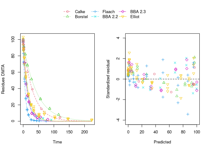
error_model = "tc", quiet = TRUE)The plot of the individual SFO fits shown below suggests that at least in some datasets the degradation slows down towards later time points, and that the scatter of the residuals error is smaller for smaller values (panel to the right):
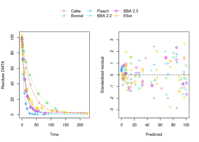
Using biexponential decline (DFOP) results in a slightly more random scatter of the residuals:

The population curve (bold line) in the above plot results from taking the mean of the individual transformed parameters, i.e. of log k1 and log k2, as well as of the logit of the g parameter of the DFOP model). Here, this procedure does not result in parameters that represent the degradation well, because in some datasets the fitted value for k2 is extremely close to zero, leading to a log k2 value that dominates the average. This is alleviated if only rate constants that pass the t-test for significant difference from zero (on the untransformed scale) are considered in the averaging:
While this is visually much more satisfactory, such an average procedure could introduce a bias, as not all results from the individual fits enter the population curve with the same weight. This is where nonlinear mixed-effects models can help out by treating all datasets with equally by fitting a parameter distribution model together with the degradation model and the error model (see below).
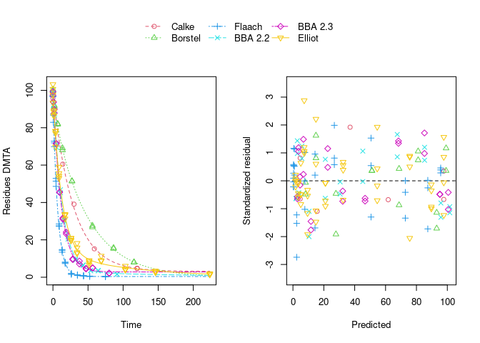
The remaining trend of the residuals to be higher for higher predicted residues is reduced by using the two-component error model:
Nonlinear mixed-effects models
Instead of taking a model selection decision for each of the individual fits, we fit nonlinear mixed-effects models (using different fitting algorithms as implemented in different packages) and do model selection using all available data at the same time. In order to make sure that these decisions are not unduly influenced by the type of algorithm used, by implementation details or by the use of wrong control parameters, we compare the model selection results obtained with different R packages, with different algorithms and checking control parameters.
nlme
The nlme package was the first R extension providing facilities to fit nonlinear mixed-effects models. We use would like to do model selection from all four combinations of degradation models and error models based on the AIC. However, fitting the DFOP model with constant variance and using default control parameters results in an error, signalling that the maximum number of 50 iterations was reached, potentially indicating overparameterisation. However, the algorithm converges when the two-component error model is used in combination with the DFOP model. This can be explained by the fact that the smaller residues observed at later sampling times get more weight when using the two-component error model which will counteract the tendency of the algorithm to try parameter combinations unsuitable for fitting these data.
library(nlme)
f_parent_nlme_sfo_const <- nlme(f_parent_mkin_const["SFO", ])
#f_parent_nlme_dfop_const <- nlme(f_parent_mkin_const["DFOP", ])
# maxIter = 50 reached
f_parent_nlme_sfo_tc <- nlme(f_parent_mkin_tc["SFO", ])
f_parent_nlme_dfop_tc <- nlme(f_parent_mkin_tc["DFOP", ])
Note that overparameterisation is also indicated by warnings obtained when fitting SFO or DFOP with the two-component error model (‘false convergence’ in the ‘LME step’ in some iterations). In addition to these fits, attempts were also made to include correlations between random effects by using the log Cholesky parameterisation of the matrix specifying them. The code used for these attempts can be made visible below.
f_parent_nlme_sfo_const_logchol <- nlme(f_parent_mkin_const["SFO", ],
  random = pdLogChol(list(DMTA_0 ~ 1, log_k_DMTA ~ 1)))
anova(f_parent_nlme_sfo_const, f_parent_nlme_sfo_const_logchol) # not better
#f_parent_nlme_dfop_tc_logchol <- update(f_parent_nlme_dfop_tc,
#  random = pdLogChol(list(DMTA_0 ~ 1, log_k1 ~ 1, log_k2 ~ 1, g_qlogis ~ 1)))
# using log Cholesky parameterisation for random effects (nlme default) does
# not converge here and gives lots of warnings about the LME step not converging
The model comparison function of the nlme package can directly be applied to these fits showing a similar goodness-of-fit of the SFO model, but a much lower AIC for the DFOP model fitted with the two-component error model. Also, the likelihood ratio test indicates that this difference is significant. as the p-value is below 0.0001.
anova(
  f_parent_nlme_sfo_const, f_parent_nlme_sfo_tc, f_parent_nlme_dfop_tc
)
Model df AIC BIC logLik Test L.Ratio p-value
f_parent_nlme_sfo_const 1 5 818.63 834.00 -404.31
f_parent_nlme_sfo_tc 2 6 820.61 839.06 -404.31 1 vs 2 0.014 0.9049
f_parent_nlme_dfop_tc 3 10 687.84 718.59 -333.92 2 vs 3 140.771 <.0001The selected model (DFOP with two-component error) fitted to the data assuming no correlations between random effects is shown below.
plot(f_parent_nlme_dfop_tc)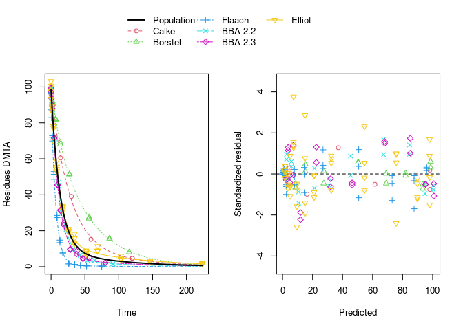
saemix
The saemix package provided the first Open Source implementation of the Stochastic Approximation to the Expectation Maximisation (SAEM) algorithm. SAEM fits of degradation models can be performed using an interface to the saemix package available in current development versions of the mkin package.
The corresponding SAEM fits of the four combinations of degradation and error models are fitted below. As there is no convergence criterion implemented in the saemix package, the convergence plots need to be manually checked for every fit.
The convergence plot for the SFO model using constant variance is shown below.
library(saemix)
f_parent_saemix_sfo_const <- mkin::saem(f_parent_mkin_const["SFO", ], quiet = TRUE,
  transformations = "saemix")
plot(f_parent_saemix_sfo_const$so, plot.type = "convergence")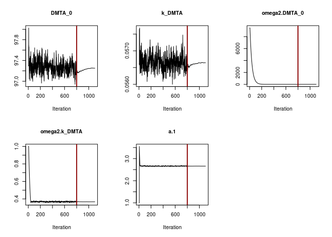
Obviously the default number of iterations is sufficient to reach convergence. This can also be said for the SFO fit using the two-component error model.
f_parent_saemix_sfo_tc <- mkin::saem(f_parent_mkin_tc["SFO", ], quiet = TRUE,
  transformations = "saemix")
plot(f_parent_saemix_sfo_tc$so, plot.type = "convergence")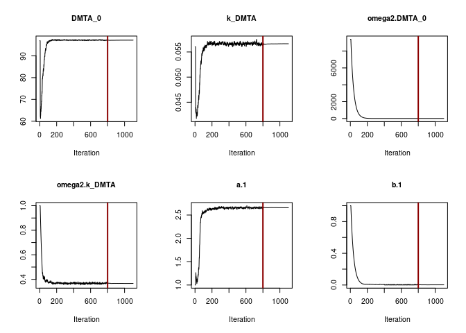
When fitting the DFOP model with constant variance, parameter convergence is not as unambiguous (see the failure of nlme with the default number of iterations above). Therefore, the number of iterations in the first phase of the algorithm was increased, leading to visually satisfying convergence.
f_parent_saemix_dfop_const <- mkin::saem(f_parent_mkin_const["DFOP", ], quiet = TRUE,
  control = saemixControl(nbiter.saemix = c(800, 200), print = FALSE,
    save = FALSE, save.graphs = FALSE, displayProgress = FALSE),
  transformations = "saemix")
plot(f_parent_saemix_dfop_const$so, plot.type = "convergence")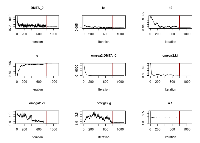
The same applies to the case where the DFOP model is fitted with the two-component error model. Convergence of the variance of k2 is enhanced by using the two-component error, it remains more or less stable already after 200 iterations of the first phase.
f_parent_saemix_dfop_tc_moreiter <- mkin::saem(f_parent_mkin_tc["DFOP", ], quiet = TRUE,
  control = saemixControl(nbiter.saemix = c(800, 200), print = FALSE,
    save = FALSE, save.graphs = FALSE, displayProgress = FALSE),
  transformations = "saemix")
plot(f_parent_saemix_dfop_tc_moreiter$so, plot.type = "convergence")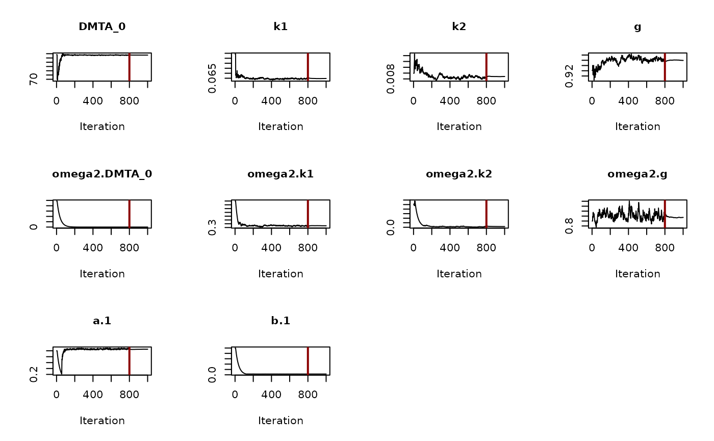
The four combinations can be compared using the model comparison function from the saemix package:
compare.saemix(f_parent_saemix_sfo_const$so, f_parent_saemix_sfo_tc$so,
  f_parent_saemix_dfop_const$so, f_parent_saemix_dfop_tc_moreiter$so)
Likelihoods calculated by importance sampling AIC BIC
1 818.37 817.33
2 820.38 819.14
3 725.91 724.04
4 683.64 681.55As in the case of nlme fits, the DFOP model fitted with two-component error (number 4) gives the lowest AIC. The numeric values are reasonably close to the ones obtained using nlme, considering that the algorithms for fitting the model and for the likelihood calculation are quite different.
In order to check the influence of the likelihood calculation algorithms implemented in saemix, the likelihood from Gaussian quadrature is added to the best fit, and the AIC values obtained from the three methods are compared.
f_parent_saemix_dfop_tc_moreiter$so <-
  llgq.saemix(f_parent_saemix_dfop_tc_moreiter$so)
AIC(f_parent_saemix_dfop_tc_moreiter$so)
[1] 683.64
AIC(f_parent_saemix_dfop_tc_moreiter$so, method = "gq")[1] 683.7
AIC(f_parent_saemix_dfop_tc_moreiter$so, method = "lin")[1] 683.17The AIC values based on importance sampling and Gaussian quadrature are quite similar. Using linearisation is less accurate, but still gives a similar value.
nlmixr
In the last years, a lot of effort has been put into the nlmixr package which is designed for pharmacokinetics, where nonlinear mixed-effects models are routinely used, but which can also be used for related data like chemical degradation data. A current development branch of the mkin package provides an interface between mkin and nlmixr. Here, we check if we get equivalent results when using a refined version of the First Order Conditional Estimation (FOCE) algorithm used in nlme, namely First Order Conditional Estimation with Interaction (FOCEI), and the SAEM algorithm as implemented in nlmixr.
First, the focei algorithm is used for the four model combinations and the goodness of fit of the results is compared.
library(nlmixr)
f_parent_nlmixr_focei_sfo_const <- nlmixr(f_parent_mkin_const["SFO", ], est = "focei")
f_parent_nlmixr_focei_sfo_tc <- nlmixr(f_parent_mkin_tc["SFO", ], est = "focei")
f_parent_nlmixr_focei_dfop_const <- nlmixr(f_parent_mkin_const["DFOP", ], est = "focei")
f_parent_nlmixr_focei_dfop_tc<- nlmixr(f_parent_mkin_tc["DFOP", ], est = "focei")
AIC(f_parent_nlmixr_focei_sfo_const$nm, f_parent_nlmixr_focei_sfo_tc$nm,
  f_parent_nlmixr_focei_dfop_const$nm, f_parent_nlmixr_focei_dfop_tc$nm)
df AIC
f_parent_nlmixr_focei_sfo_const$nm 5 818.63
f_parent_nlmixr_focei_sfo_tc$nm 6 820.61
f_parent_nlmixr_focei_dfop_const$nm 9 728.11
f_parent_nlmixr_focei_dfop_tc$nm 10 687.82The AIC values are very close to the ones obtained with nlme which are repeated below for convenience.
AIC(
  f_parent_nlme_sfo_const, f_parent_nlme_sfo_tc, f_parent_nlme_dfop_tc
)
df AIC
f_parent_nlme_sfo_const 5 818.63
f_parent_nlme_sfo_tc 6 820.61
f_parent_nlme_dfop_tc 10 687.84Secondly, we use the SAEM estimation routine and check the convergence plots for SFO with constant variance
f_parent_nlmixr_saem_sfo_const <- nlmixr(f_parent_mkin_const["SFO", ], est = "saem",
  control = nlmixr::saemControl(logLik = TRUE))
traceplot(f_parent_nlmixr_saem_sfo_const$nm)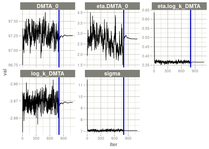
for SFO with two-component error
f_parent_nlmixr_saem_sfo_tc <- nlmixr(f_parent_mkin_tc["SFO", ], est = "saem",
  control = nlmixr::saemControl(logLik = TRUE))
traceplot(f_parent_nlmixr_saem_sfo_tc$nm)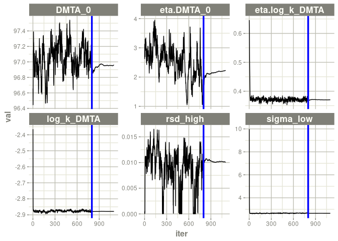
For DFOP with constant variance, the convergence plots show considerable instability of the fit, which can be alleviated by increasing the number of iterations and the number of parallel chains for the first phase of algorithm.
f_parent_nlmixr_saem_dfop_const <- nlmixr(f_parent_mkin_const["DFOP", ], est = "saem",
  control = nlmixr::saemControl(logLik = TRUE, nBurn = 1000), nmc = 15)
traceplot(f_parent_nlmixr_saem_dfop_const$nm)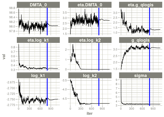
For DFOP with two-component error, the same increase in iterations and parallel chains was used, but using the two-component error appears to lead to a less erratic convergence, so this may not be necessary to this degree.
f_parent_nlmixr_saem_dfop_tc <- nlmixr(f_parent_mkin_tc["DFOP", ], est = "saem",
  control = nlmixr::saemControl(logLik = TRUE, nBurn = 1000, nmc = 15))
traceplot(f_parent_nlmixr_saem_dfop_tc$nm)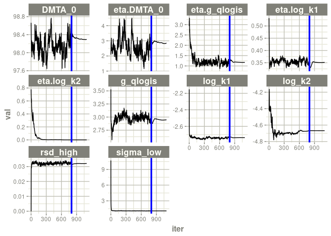
The AIC values are internally calculated using Gaussian quadrature. For an unknown reason, the AIC value obtained for the DFOP fit using the two-component error model is given as Infinity.
AIC(f_parent_nlmixr_saem_sfo_const$nm, f_parent_nlmixr_saem_sfo_tc$nm,
  f_parent_nlmixr_saem_dfop_const$nm, f_parent_nlmixr_saem_dfop_tc$nm)
df AIC
f_parent_nlmixr_saem_sfo_const$nm 5 820.54
f_parent_nlmixr_saem_sfo_tc$nm 6 835.26
f_parent_nlmixr_saem_dfop_const$nm 9 842.84
f_parent_nlmixr_saem_dfop_tc$nm 10 684.51The following table gives the AIC values obtained with the three packages.
AIC_all <- data.frame(
  "Degradation model" = c("SFO", "SFO", "DFOP", "DFOP"),
  "Error model" = c("const", "tc", "const", "tc"),
  nlme = c(AIC(f_parent_nlme_sfo_const), AIC(f_parent_nlme_sfo_tc), NA, AIC(f_parent_nlme_dfop_tc)),
  nlmixr_focei = sapply(list(f_parent_nlmixr_focei_sfo_const$nm, f_parent_nlmixr_focei_sfo_tc$nm,
  f_parent_nlmixr_focei_dfop_const$nm, f_parent_nlmixr_focei_dfop_tc$nm), AIC),
  saemix = sapply(list(f_parent_saemix_sfo_const$so, f_parent_saemix_sfo_tc$so,
    f_parent_saemix_dfop_const$so, f_parent_saemix_dfop_tc_moreiter$so), AIC),
  nlmixr_saem = sapply(list(f_parent_nlmixr_saem_sfo_const$nm, f_parent_nlmixr_saem_sfo_tc$nm,
  f_parent_nlmixr_saem_dfop_const$nm, f_parent_nlmixr_saem_dfop_tc$nm), AIC)
)
kable(AIC_all)| Degradation.model | Error.model | nlme | nlmixr_focei | saemix | nlmixr_saem |
|---|---|---|---|---|---|
| SFO | const | 818.63 | 818.63 | 818.37 | 820.54 |
| SFO | tc | 820.61 | 820.61 | 820.38 | 835.26 |
| DFOP | const | NA | 728.11 | 725.91 | 842.84 |
| DFOP | tc | 687.84 | 687.82 | 683.64 | 684.51 |
References
EFSA. 2018. “Peer Review of the Pesticide Risk Assessment of the Active Substance Dimethenamid-P.” EFSA Journal 16 (4): 5211.
Rapporteur Member State Germany, Co-Rapporteur Member State Bulgaria. 2018. “Renewal Assessment Report Dimethenamid-P Volume 3 - B.8 Environmental fate and behaviour, Rev. 2 - November 2017.” https://open.efsa.europa.eu/study-inventory/EFSA-Q-2014-00716.