Create an nlme model for an mmkin row object

This functions sets up a nonlinear mixed effects model for an mmkin row object. An mmkin row object is essentially a list of mkinfit objects that have been obtained by fitting the same model to a list of datasets.

# S3 method for mmkin
nlme(
  model,
  data = sys.frame(sys.parent()),
  fixed,
  random = fixed,
  groups,
  start,
  correlation = NULL,
  weights = NULL,
  subset,
  method = c("ML", "REML"),
  na.action = na.fail,
  naPattern,
  control = list(),
  verbose = FALSE
)

# S3 method for nlme.mmkin
print(x, ...)

# S3 method for nlme.mmkin
update(object, ...)

Arguments

model	An mmkin row object.
data	Ignored, data are taken from the mmkin model
fixed	Ignored, all degradation parameters fitted in the mmkin model are used as fixed parameters
random	If not specified, all fixed effects are complemented with uncorrelated random effects
groups	See the documentation of nlme
start	If not specified, mean values of the fitted degradation parameters taken from the mmkin object are used
correlation	See the documentation of nlme
weights	passed to nlme
subset	passed to nlme
method	passed to nlme
na.action	passed to nlme
naPattern	passed to nlme
control	passed to nlme
verbose	passed to nlme
x	An nlme.mmkin object to print
...	Update specifications passed to update.nlme
object	An nlme.mmkin object to update

Value

Upon success, a fitted nlme.mmkin object, which is an nlme object with additional elements

Note

As the object inherits from nlme::nlme, there is a wealth of methods that will automatically work on 'nlme.mmkin' objects, such as nlme::intervals(), nlme::anova.lme() and nlme::coef.lme().

Examples

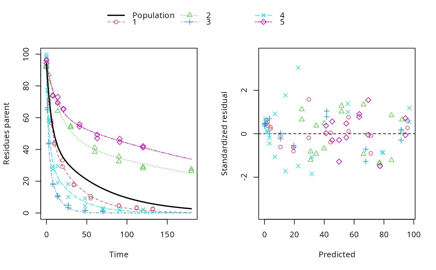
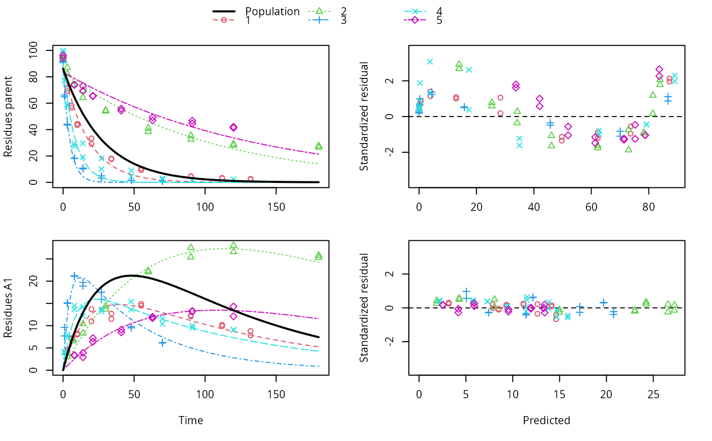
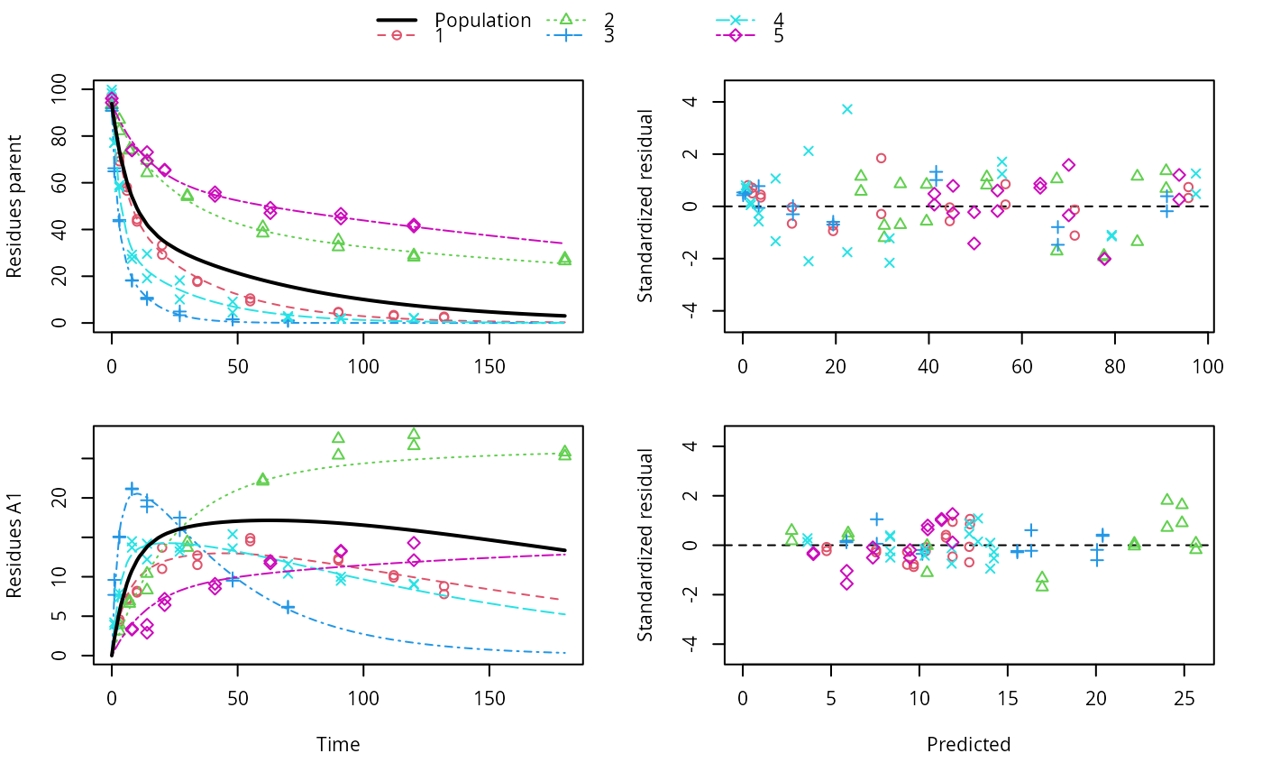
ds <- lapply(experimental_data_for_UBA_2019[6:10],
 function(x) subset(x$data[c("name", "time", "value")], name == "parent"))
f <- mmkin(c("SFO", "DFOP"), ds, quiet = TRUE, cores = 1)
library(nlme)
f_nlme_sfo <- nlme(f["SFO", ])
f_nlme_dfop <- nlme(f["DFOP", ])
AIC(f_nlme_sfo, f_nlme_dfop)
#>             df      AIC
#> f_nlme_sfo   5 625.0539
#> f_nlme_dfop  9 495.1270
print(f_nlme_dfop)
#> Kinetic nonlinear mixed-effects model fit by maximum likelihood
#> 
#> Structural model:
#> d_parent/dt = - ((k1 * g * exp(-k1 * time) + k2 * (1 - g) * exp(-k2 *
#>            time)) / (g * exp(-k1 * time) + (1 - g) * exp(-k2 * time)))
#>            * parent
#> 
#> Data:
#> 90 observations of 1 variable(s) grouped in 5 datasets
#> 
#> Log-likelihood: -238.5635
#> 
#> Fixed effects:
#>  list(parent_0 ~ 1, log_k1 ~ 1, log_k2 ~ 1, g_ilr ~ 1) 
#>    parent_0      log_k1      log_k2       g_ilr 
#> 94.17015133 -1.80015306 -4.14738870  0.02290935 
#> 
#> Random effects:
#>  Formula: list(parent_0 ~ 1, log_k1 ~ 1, log_k2 ~ 1, g_ilr ~ 1)
#>  Level: ds
#>  Structure: Diagonal
#>         parent_0    log_k1  log_k2     g_ilr Residual
#> StdDev: 2.488249 0.8447273 1.32965 0.3289311 2.321364
#> 
plot(f_nlme_dfop)
endpoints(f_nlme_dfop)
#> $distimes
#>            DT50     DT90 DT50back  DT50_k1  DT50_k2
#> parent 10.79857 100.7937 30.34193 4.193938 43.85443
#> 

# \dontrun{
  f_nlme_2 <- nlme(f["SFO", ], start = c(parent_0 = 100, log_k_parent = 0.1))
  update(f_nlme_2, random = parent_0 ~ 1)
#> Kinetic nonlinear mixed-effects model fit by maximum likelihood
#> 
#> Structural model:
#> d_parent/dt = - k_parent * parent
#> 
#> Data:
#>  observations of 0 variable(s) grouped in 0 datasets
#> 
#> Log-likelihood: -404.3729
#> 
#> Fixed effects:
#>  list(parent_0 ~ 1, log_k_parent ~ 1) 
#>     parent_0 log_k_parent 
#>    75.933480    -3.555983 
#> 
#> Random effects:
#>  Formula: parent_0 ~ 1 | ds
#>            parent_0 Residual
#> StdDev: 0.002416792 21.63027
#> 
  ds_2 <- lapply(experimental_data_for_UBA_2019[6:10],
   function(x) x$data[c("name", "time", "value")])
  m_sfo_sfo <- mkinmod(parent = mkinsub("SFO", "A1"),
    A1 = mkinsub("SFO"), use_of_ff = "min", quiet = TRUE)
  m_sfo_sfo_ff <- mkinmod(parent = mkinsub("SFO", "A1"),
    A1 = mkinsub("SFO"), use_of_ff = "max", quiet = TRUE)
  m_dfop_sfo <- mkinmod(parent = mkinsub("DFOP", "A1"),
    A1 = mkinsub("SFO"), quiet = TRUE)

  f_2 <- mmkin(list("SFO-SFO" = m_sfo_sfo,
   "SFO-SFO-ff" = m_sfo_sfo_ff,
   "DFOP-SFO" = m_dfop_sfo),
    ds_2, quiet = TRUE)

  f_nlme_sfo_sfo <- nlme(f_2["SFO-SFO", ])
  plot(f_nlme_sfo_sfo)

  # With formation fractions
  f_nlme_sfo_sfo_ff <- nlme(f_2["SFO-SFO-ff", ])
  plot(f_nlme_sfo_sfo_ff)

  # For the following fit we need to increase pnlsMaxIter and the tolerance
  # to get convergence
  f_nlme_dfop_sfo <- nlme(f_2["DFOP-SFO", ],
    control = list(pnlsMaxIter = 120, tolerance = 5e-4), verbose = TRUE)
#> 
#> **Iteration 1
#> LME step: Loglik: -404.9582, nlminb iterations: 1
#> reStruct  parameters:
#>        ds1        ds2        ds3        ds4        ds5        ds6 
#> -0.4114355  0.9798697  1.6990037  0.7293315  0.3354323  1.7113046 
#>  Beginning PNLS step: ..  completed fit_nlme() step.
#> PNLS step: RSS =  630.3644 
#>  fixed effects: 93.82269  -5.455991  -0.6788957  -1.862196  -4.199671  0.05532828  
#>  iterations: 120 
#> Convergence crit. (must all become <= tolerance = 0.0005):
#>     fixed  reStruct 
#> 0.7885368 0.5822683 
#> 
#> **Iteration 2
#> LME step: Loglik: -407.7755, nlminb iterations: 11
#> reStruct  parameters:
#>          ds1          ds2          ds3          ds4          ds5          ds6 
#> -0.371224133  0.003056179  1.789939402  0.724671158  0.301602977  1.754200729 
#>  Beginning PNLS step: ..  completed fit_nlme() step.
#> PNLS step: RSS =  630.3633 
#>  fixed effects: 93.82269  -5.455992  -0.6788958  -1.862196  -4.199671  0.05532831  
#>  iterations: 120 
#> Convergence crit. (must all become <= tolerance = 0.0005):
#>        fixed     reStruct 
#> 4.789774e-07 2.200661e-05 

  plot(f_nlme_dfop_sfo)

  anova(f_nlme_dfop_sfo, f_nlme_sfo_sfo)
#>                 Model df       AIC       BIC    logLik   Test  L.Ratio p-value
#> f_nlme_dfop_sfo     1 13  843.8547  884.6201 -408.9273                        
#> f_nlme_sfo_sfo      2  9 1085.1821 1113.4043 -533.5910 1 vs 2 249.3274  <.0001

  endpoints(f_nlme_sfo_sfo)
#> $ff
#> parent_sink   parent_A1     A1_sink 
#>   0.5912432   0.4087568   1.0000000 
#> 
#> $distimes
#>            DT50     DT90
#> parent 19.13518  63.5657
#> A1     66.02155 219.3189
#> 
  endpoints(f_nlme_dfop_sfo)
#> $ff
#>   parent_A1 parent_sink 
#>   0.2768574   0.7231426 
#> 
#> $distimes
#>             DT50     DT90 DT50back  DT50_k1  DT50_k2
#> parent  11.07091 104.6320 31.49738 4.462384 46.20825
#> A1     162.30536 539.1667       NA       NA       NA
#> 

  if (length(findFunction("varConstProp")) > 0) { # tc error model for nlme available
    # Attempts to fit metabolite kinetics with the tc error model are possible,
    # but need tweeking of control values and sometimes do not converge

    f_tc <- mmkin(c("SFO", "DFOP"), ds, quiet = TRUE, error_model = "tc")
    f_nlme_sfo_tc <- nlme(f_tc["SFO", ])
    f_nlme_dfop_tc <- nlme(f_tc["DFOP", ])
    AIC(f_nlme_sfo, f_nlme_sfo_tc, f_nlme_dfop, f_nlme_dfop_tc)
    print(f_nlme_dfop_tc)
  }
#> Kinetic nonlinear mixed-effects model fit by maximum likelihood
#> 
#> Structural model:
#> d_parent/dt = - ((k1 * g * exp(-k1 * time) + k2 * (1 - g) * exp(-k2 *
#>            time)) / (g * exp(-k1 * time) + (1 - g) * exp(-k2 * time)))
#>            * parent
#> 
#> Data:
#> 90 observations of 1 variable(s) grouped in 5 datasets
#> 
#> Log-likelihood: -238.4298
#> 
#> Fixed effects:
#>  list(parent_0 ~ 1, log_k1 ~ 1, log_k2 ~ 1, g_ilr ~ 1) 
#>    parent_0      log_k1      log_k2       g_ilr 
#> 94.04774463 -1.82339924 -4.16715509  0.04020161 
#> 
#> Random effects:
#>  Formula: list(parent_0 ~ 1, log_k1 ~ 1, log_k2 ~ 1, g_ilr ~ 1)
#>  Level: ds
#>  Structure: Diagonal
#>         parent_0    log_k1   log_k2     g_ilr Residual
#> StdDev: 2.473883 0.8499901 1.337187 0.3294411        1
#> 
#> Variance function:
#>  Structure: Constant plus proportion of variance covariate
#>  Formula: ~fitted(.) 
#>  Parameter estimates:
#>      const       prop 
#> 2.23222625 0.01262414 

  f_2_obs <- mmkin(list("SFO-SFO" = m_sfo_sfo,
   "DFOP-SFO" = m_dfop_sfo),
    ds_2, quiet = TRUE, error_model = "obs")
  f_nlme_sfo_sfo_obs <- nlme(f_2_obs["SFO-SFO", ])
  print(f_nlme_sfo_sfo_obs)
#> Kinetic nonlinear mixed-effects model fit by maximum likelihood
#> 
#> Structural model:
#> d_parent/dt = - k_parent_sink * parent - k_parent_A1 * parent
#> d_A1/dt = + k_parent_A1 * parent - k_A1_sink * A1
#> 
#> Data:
#> 170 observations of 2 variable(s) grouped in 5 datasets
#> 
#> Log-likelihood: -472.976
#> 
#> Fixed effects:
#>  list(parent_0 ~ 1, log_k_parent_sink ~ 1, log_k_parent_A1 ~ 1,      log_k_A1_sink ~ 1) 
#>          parent_0 log_k_parent_sink   log_k_parent_A1     log_k_A1_sink 
#>         87.975536         -3.669816         -4.164127         -4.645073 
#> 
#> Random effects:
#>  Formula: list(parent_0 ~ 1, log_k_parent_sink ~ 1, log_k_parent_A1 ~ 1,      log_k_A1_sink ~ 1)
#>  Level: ds
#>  Structure: Diagonal
#>         parent_0 log_k_parent_sink log_k_parent_A1 log_k_A1_sink Residual
#> StdDev: 3.992214           1.77702        1.054733     0.4821383 6.482585
#> 
#> Variance function:
#>  Structure: Different standard deviations per stratum
#>  Formula: ~1 | name 
#>  Parameter estimates:
#>    parent        A1 
#> 1.0000000 0.2050003 
  # The same with DFOP-SFO does not converge, apparently the variances of
  # parent and A1 are too similar in this case, so that the model is
  # overparameterised
  #f_nlme_dfop_sfo_obs <- nlme(f_2_obs["DFOP-SFO", ], control = list(maxIter = 100))
# }

Create an nlme model for an mmkin row object

Arguments

Value

Note

See also

Examples