Fit nonlinear mixed models with SAEM

This function uses saemix::saemix() as a backend for fitting nonlinear mixed effects models created from mmkin row objects using the Stochastic Approximation Expectation Maximisation algorithm (SAEM).

saem(object, control, ...)

# S3 method for mmkin
saem(
  object,
  control = list(displayProgress = FALSE, print = FALSE, save = FALSE, save.graphs =
    FALSE),
  cores = 1,
  verbose = FALSE,
  suppressPlot = TRUE,
  quiet = FALSE,
  ...
)

# S3 method for saem.mmkin
print(x, digits = max(3, getOption("digits") - 3), ...)

saemix_model(object, cores = 1, verbose = FALSE, ...)

saemix_data(object, verbose = FALSE, ...)

Arguments

object	An mmkin row object containing several fits of the same mkinmod model to different datasets
control	Passed to saemix::saemix
...	Further parameters passed to saemix::saemixModel.
cores	The number of cores to be used for multicore processing using `parallel::mclapply()`. Using more than 1 core is experimental and may lead to excessive forking, apparently depending on the BLAS version used.
verbose	Should we print information about created objects of type saemix::SaemixModel and saemix::SaemixData?
suppressPlot	Should we suppress any plotting that is done by the saemix function?
quiet	Should we suppress the messages saemix prints at the beginning and the end of the optimisation process?
x	An saem.mmkin object to print
digits	Number of digits to use for printing

Value

An S3 object of class 'saem.mmkin', containing the fitted saemix::SaemixObject as a list component named 'so'. The object also inherits from 'mixed.mmkin'.

An saemix::SaemixModel object.

An saemix::SaemixData object.

Details

An mmkin row object is essentially a list of mkinfit objects that have been obtained by fitting the same model to a list of datasets using mkinfit.

Starting values for the fixed effects (population mean parameters, argument psi0 of saemix::saemixModel() are the mean values of the parameters found using mmkin.

Examples

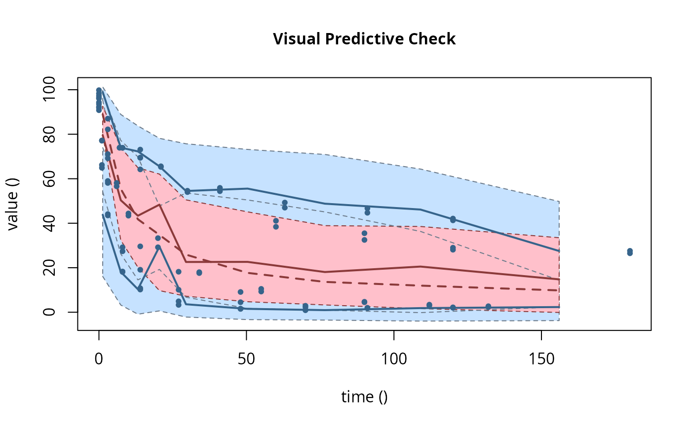
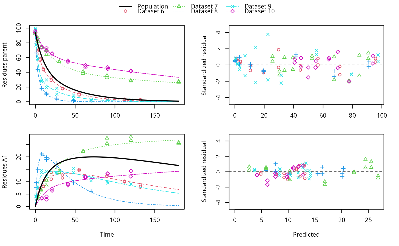
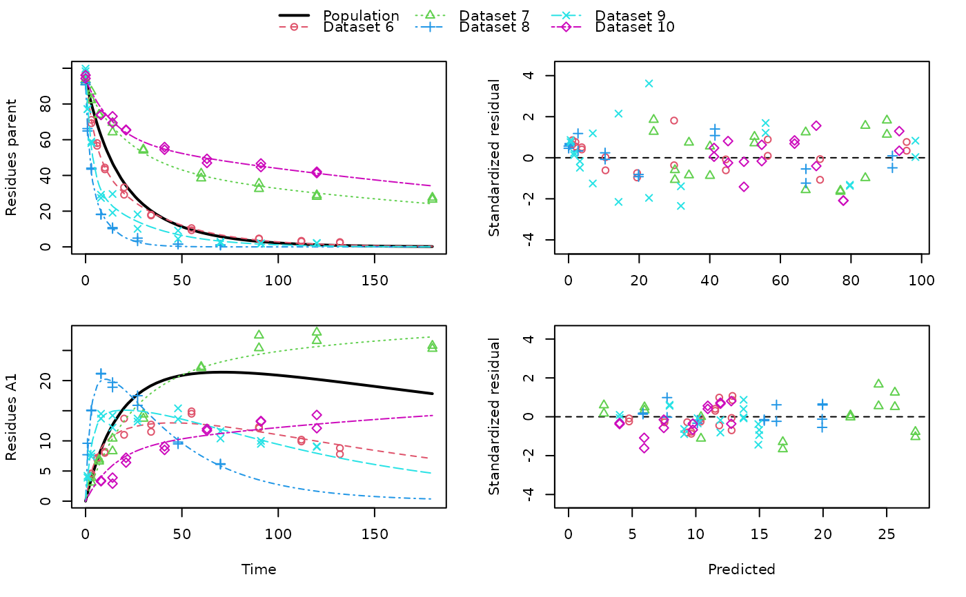
# \dontrun{
ds <- lapply(experimental_data_for_UBA_2019[6:10],
 function(x) subset(x$data[c("name", "time", "value")]))
names(ds) <- paste("Dataset", 6:10)
f_mmkin_parent_p0_fixed <- mmkin("FOMC", ds, cores = 1,
  state.ini = c(parent = 100), fixed_initials = "parent", quiet = TRUE)
f_saem_p0_fixed <- saem(f_mmkin_parent_p0_fixed)
#> Running main SAEM algorithm
#> [1] "Wed Nov 11 19:47:58 2020"
#> ....
#>     Minimisation finished
#> [1] "Wed Nov 11 19:48:00 2020"

f_mmkin_parent <- mmkin(c("SFO", "FOMC", "DFOP"), ds, quiet = TRUE)
f_saem_sfo <- saem(f_mmkin_parent["SFO", ])
#> Running main SAEM algorithm
#> [1] "Wed Nov 11 19:48:01 2020"
#> ....
#>     Minimisation finished
#> [1] "Wed Nov 11 19:48:03 2020"
f_saem_fomc <- saem(f_mmkin_parent["FOMC", ])
#> Running main SAEM algorithm
#> [1] "Wed Nov 11 19:48:03 2020"
#> ....
#>     Minimisation finished
#> [1] "Wed Nov 11 19:48:05 2020"
f_saem_dfop <- saem(f_mmkin_parent["DFOP", ])
#> Running main SAEM algorithm
#> [1] "Wed Nov 11 19:48:06 2020"
#> ....
#>     Minimisation finished
#> [1] "Wed Nov 11 19:48:08 2020"

# The returned saem.mmkin object contains an SaemixObject, therefore we can use
# functions from saemix
library(saemix)
#> Package saemix, version 3.1.9000
#>   please direct bugs, questions and feedback to emmanuelle.comets@inserm.fr
compare.saemix(list(f_saem_sfo$so, f_saem_fomc$so, f_saem_dfop$so))
#> Likelihoods computed by importance sampling 
#>        AIC      BIC
#> 1 624.2484 622.2956
#> 2 467.7096 464.9757
#> 3 495.4373 491.9222
plot(f_saem_fomc$so, plot.type = "convergence")
#> Plotting convergence plots
plot(f_saem_fomc$so, plot.type = "individual.fit")
#> Plotting individual fits
plot(f_saem_fomc$so, plot.type = "npde")
#> Simulating data using nsim = 1000 simulated datasets
#> Computing WRES and npde .
#> Plotting npde
#> ---------------------------------------------
#> Distribution of npde:
#>            mean= -0.01528   (SE= 0.098 )
#>        variance= 0.862   (SE= 0.13 )
#>        skewness= 0.5016 
#>        kurtosis= 1.18 
#> ---------------------------------------------
#> 
#> Statistical tests
#>   Wilcoxon signed rank test  : 0.679
#>   Fisher variance test       : 0.36
#>   SW test of normality       : 0.0855 .
#> Global adjusted p-value      : 0.257
#> ---
#> Signif. codes: '***' 0.001 '**' 0.01 '*' 0.05 '.' 0.1 
#> ---------------------------------------------
plot(f_saem_fomc$so, plot.type = "vpc")
#> Performing simulations under the model.
#> Plotting VPC
#> Method used for VPC: binning by quantiles on X , dividing into the following intervals
#>   Interval  Centered.On
#> 1 (-1,3]      1.3      
#> 2 (3,8]       7.4      
#> 3 (8,14]     13.2      
#> 4 (14,21]    20.5      
#> 5 (21,37.7]  29.5      
#> 6 (37.7,60]  50.4      
#> 7 (60,90]    76.6      
#> 8 (90,120]  109.0      
#> 9 (120,180] 156.0      

f_mmkin_parent_tc <- update(f_mmkin_parent, error_model = "tc")
f_saem_fomc_tc <- saem(f_mmkin_parent_tc["FOMC", ])
#> Running main SAEM algorithm
#> [1] "Wed Nov 11 19:48:11 2020"
#> ....
#>     Minimisation finished
#> [1] "Wed Nov 11 19:48:16 2020"
compare.saemix(list(f_saem_fomc$so, f_saem_fomc_tc$so))
#> Likelihoods computed by importance sampling 
#>        AIC      BIC
#> 1 467.7096 464.9757
#> 2 469.5208 466.3963

sfo_sfo <- mkinmod(parent = mkinsub("SFO", "A1"),
  A1 = mkinsub("SFO"))
#> Successfully compiled differential equation model from auto-generated C code.
fomc_sfo <- mkinmod(parent = mkinsub("FOMC", "A1"),
  A1 = mkinsub("SFO"))
#> Successfully compiled differential equation model from auto-generated C code.
dfop_sfo <- mkinmod(parent = mkinsub("DFOP", "A1"),
  A1 = mkinsub("SFO"))
#> Successfully compiled differential equation model from auto-generated C code.
# The following fit uses analytical solutions for SFO-SFO and DFOP-SFO,
# and compiled ODEs for FOMC, both are fast
f_mmkin <- mmkin(list(
    "SFO-SFO" = sfo_sfo, "FOMC-SFO" = fomc_sfo, "DFOP-SFO" = dfop_sfo),
  ds, quiet = TRUE)
# These take about five seconds each on this system, as we use
# analytical solutions written for saemix. When using the analytical
# solutions written for mkin this took around four minutes
f_saem_sfo_sfo <- saem(f_mmkin["SFO-SFO", ])
#> Running main SAEM algorithm
#> [1] "Wed Nov 11 19:48:18 2020"
#> ....
#>     Minimisation finished
#> [1] "Wed Nov 11 19:48:23 2020"
f_saem_dfop_sfo <- saem(f_mmkin["DFOP-SFO", ])
#> Running main SAEM algorithm
#> [1] "Wed Nov 11 19:48:23 2020"
#> ....
#>     Minimisation finished
#> [1] "Wed Nov 11 19:48:32 2020"
# We can use print, plot and summary methods to check the results
print(f_saem_dfop_sfo)
#> Kinetic nonlinear mixed-effects model fit by SAEM
#> Structural model:
#> d_parent/dt = - ((k1 * g * exp(-k1 * time) + k2 * (1 - g) * exp(-k2 *
#>            time)) / (g * exp(-k1 * time) + (1 - g) * exp(-k2 * time)))
#>            * parent
#> d_A1/dt = + f_parent_to_A1 * ((k1 * g * exp(-k1 * time) + k2 * (1 - g)
#>            * exp(-k2 * time)) / (g * exp(-k1 * time) + (1 - g) *
#>            exp(-k2 * time))) * parent - k_A1 * A1
#> 
#> Data:
#> 170 observations of 2 variable(s) grouped in 5 datasets
#> 
#> Likelihood computed by importance sampling
#>                           
#> LL by is "-407.78 (df=13)"
#>     AIC   BIC logLik
#>   841.6 836.5 -407.8
#> 
#> Fitted parameters:
#>                     estimate    lower   upper
#> parent_0            93.76647 91.15312 96.3798
#> log_k_A1            -6.13235 -8.45788 -3.8068
#> f_parent_qlogis     -0.97364 -1.36940 -0.5779
#> log_k1              -2.53176 -3.80372 -1.2598
#> log_k2              -3.58667 -5.29524 -1.8781
#> g_qlogis             0.01238 -1.07968  1.1044
#> Var.parent_0         7.61106 -3.34955 18.5717
#> Var.log_k_A1         4.64679 -2.73133 12.0249
#> Var.f_parent_qlogis  0.19693 -0.05498  0.4488
#> Var.log_k1           2.01717 -0.51980  4.5542
#> Var.log_k2           3.63412 -0.92964  8.1979
#> Var.g_qlogis         0.20045 -0.97425  1.3751
#> a.1                  1.88335  1.66636  2.1004
#> SD.parent_0          2.75881  0.77234  4.7453
#> SD.log_k_A1          2.15564  0.44429  3.8670
#> SD.f_parent_qlogis   0.44377  0.15994  0.7276
#> SD.log_k1            1.42027  0.52714  2.3134
#> SD.log_k2            1.90634  0.70934  3.1033
#> SD.g_qlogis          0.44771 -0.86417  1.7596
plot(f_saem_dfop_sfo)
summary(f_saem_dfop_sfo, data = FALSE)
#>                           
#> LL by is "-407.78 (df=13)"
#> saemix version used for fitting:      3.1.9000 
#> mkin version used for pre-fitting:  0.9.50.4 
#> R version used for fitting:         4.0.3 
#> Date of fit:     Wed Nov 11 19:48:33 2020 
#> Date of summary: Wed Nov 11 19:48:33 2020 
#> 
#> Equations:
#> d_parent/dt = - ((k1 * g * exp(-k1 * time) + k2 * (1 - g) * exp(-k2 *
#>            time)) / (g * exp(-k1 * time) + (1 - g) * exp(-k2 * time)))
#>            * parent
#> d_A1/dt = + f_parent_to_A1 * ((k1 * g * exp(-k1 * time) + k2 * (1 - g)
#>            * exp(-k2 * time)) / (g * exp(-k1 * time) + (1 - g) *
#>            exp(-k2 * time))) * parent - k_A1 * A1
#> 
#> Data:
#> 170 observations of 2 variable(s) grouped in 5 datasets
#> 
#> Model predictions using solution type analytical 
#> 
#> Fitted in 9.564 s using 300, 100 iterations
#> 
#> Variance model: Constant variance 
#> 
#> Mean of starting values for individual parameters:
#>        parent_0        log_k_A1 f_parent_qlogis          log_k1          log_k2 
#>      93.8101519      -9.7647455      -0.9711148      -1.8799371      -4.2708142 
#>        g_qlogis 
#>       0.1356441 
#> 
#> Fixed degradation parameter values:
#> None
#> 
#> Results:
#> 
#> Likelihood computed by importance sampling
#>     AIC   BIC logLik
#>   841.6 836.5 -407.8
#> 
#> Optimised, transformed parameters with symmetric confidence intervals:
#>                     est.  lower   upper
#> parent_0        93.76647 91.153 96.3798
#> log_k_A1        -6.13235 -8.458 -3.8068
#> f_parent_qlogis -0.97364 -1.369 -0.5779
#> log_k1          -2.53176 -3.804 -1.2598
#> log_k2          -3.58667 -5.295 -1.8781
#> g_qlogis         0.01238 -1.080  1.1044
#> 
#> Correlation: 
#>                 prnt_0 lg__A1 f_prn_ log_k1 log_k2
#> log_k_A1        -0.013                            
#> f_parent_qlogis -0.025  0.050                     
#> log_k1           0.030  0.000 -0.005              
#> log_k2           0.010  0.005 -0.003  0.032       
#> g_qlogis        -0.063 -0.015  0.010 -0.167 -0.177
#> 
#> Random effects:
#>                      est.   lower  upper
#> SD.parent_0        2.7588  0.7723 4.7453
#> SD.log_k_A1        2.1556  0.4443 3.8670
#> SD.f_parent_qlogis 0.4438  0.1599 0.7276
#> SD.log_k1          1.4203  0.5271 2.3134
#> SD.log_k2          1.9063  0.7093 3.1033
#> SD.g_qlogis        0.4477 -0.8642 1.7596
#> 
#> Variance model:
#>      est. lower upper
#> a.1 1.883 1.666   2.1
#> 
#> Backtransformed parameters with asymmetric confidence intervals:
#>                     est.     lower    upper
#> parent_0       93.766473 9.115e+01 96.37983
#> k_A1            0.002171 2.122e-04  0.02222
#> f_parent_to_A1  0.274156 2.027e-01  0.35942
#> k1              0.079519 2.229e-02  0.28371
#> k2              0.027691 5.015e-03  0.15288
#> g               0.503095 2.536e-01  0.75109
#> 
#> Resulting formation fractions:
#>                 ff
#> parent_A1   0.2742
#> parent_sink 0.7258
#> 
#> Estimated disappearance times:
#>          DT50    DT90 DT50back DT50_k1 DT50_k2
#> parent  14.11   59.53    17.92   8.717   25.03
#> A1     319.21 1060.38       NA      NA      NA

# Using a single core, the following takes about 6 minutes as we do not have an
# analytical solution. Using 10 cores it is slower instead of faster
#f_saem_fomc <- saem(f_mmkin["FOMC-SFO", ], cores = 1)
# }

Fit nonlinear mixed models with SAEM

Arguments

Value

Details

See also

Examples