Logistic kinetics

Function describing exponential decline from a defined starting value, with an increasing rate constant, supposedly caused by microbial growth

logistic.solution(t, parent.0, kmax, k0, r)

Arguments

t	Time.
parent.0	Starting value for the response variable at time zero.
kmax	Maximum rate constant.
k0	Minumum rate constant effective at time zero.
r	Growth rate of the increase in the rate constant.

Note

The solution of the logistic model reduces to the SFO.solution if k0 is equal to kmax.

Value

The value of the response variable at time t.

References

FOCUS (2014) “Generic guidance for Estimating Persistence and Degradation Kinetics from Environmental Fate Studies on Pesticides in EU Registration” Report of the FOCUS Work Group on Degradation Kinetics, Version 1.1, 18 December 2014 http://esdac.jrc.ec.europa.eu/projects/degradation-kinetics

Examples

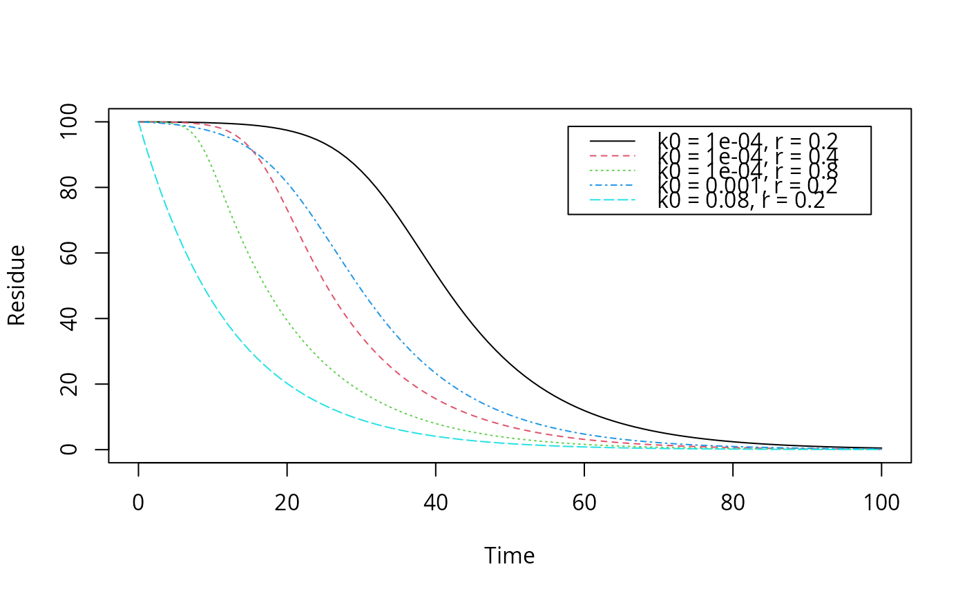
  # Reproduce the plot on page 57 of FOCUS (2014)
  plot(function(x) logistic.solution(x, 100, 0.08, 0.0001, 0.2),
       from = 0, to = 100, ylim = c(0, 100),
       xlab = "Time", ylab = "Residue")
  plot(function(x) logistic.solution(x, 100, 0.08, 0.0001, 0.4),
       from = 0, to = 100, add = TRUE, lty = 2, col = 2)
  plot(function(x) logistic.solution(x, 100, 0.08, 0.0001, 0.8),
       from = 0, to = 100, add = TRUE, lty = 3, col = 3)
  plot(function(x) logistic.solution(x, 100, 0.08, 0.001, 0.2),
       from = 0, to = 100, add = TRUE, lty = 4, col = 4)
  plot(function(x) logistic.solution(x, 100, 0.08, 0.08, 0.2),
       from = 0, to = 100, add = TRUE, lty = 5, col = 5)
  legend("topright", inset = 0.05,
         legend = paste0("k0 = ", c(0.0001, 0.0001, 0.0001, 0.001, 0.08),
                         ", r = ", c(0.2, 0.4, 0.8, 0.2, 0.2)),
         lty = 1:5, col = 1:5)

  # Fit with synthetic data
  logistic <- mkinmod(parent = mkinsub("logistic"))

  sampling_times = c(0, 1, 3, 7, 14, 28, 60, 90, 120)
  parms_logistic <- c(kmax = 0.08, k0 = 0.0001, r = 0.2)
  parms_logistic_optim <- c(parent_0 = 100, parms_logistic)
  d_logistic <- mkinpredict(logistic,
    parms_logistic, c(parent = 100),
    sampling_times)
  d_2_1 <- add_err(d_logistic,
    sdfunc = function(x) sigma_twocomp(x, 0.5, 0.07),
    n = 1, reps = 2, digits = 5, LOD = 0.1, seed = 123456)[[1]]

  m <- mkinfit("logistic", d_2_1)
#> Model cost at call  1 :  789.6044 
#> Model cost at call  2 :  789.6043 
#> Model cost at call  7 :  716.9934 
#> Model cost at call  12 :  697.1186 
#> Model cost at call  15 :  697.1185 
#> Model cost at call  16 :  697.1184 
#> Model cost at call  17 :  661.1574 
#> Model cost at call  20 :  661.1573 
#> Model cost at call  22 :  620.0542 
#> Model cost at call  25 :  620.0541 
#> Model cost at call  29 :  616.6874 
#> Model cost at call  32 :  616.6874 
#> Model cost at call  33 :  616.6874 
#> Model cost at call  34 :  615.1671 
#> Model cost at call  37 :  615.1671 
#> Model cost at call  39 :  612.0795 
#> Model cost at call  42 :  612.0795 
#> Model cost at call  43 :  612.0795 
#> Model cost at call  44 :  605.9119 
#> Model cost at call  45 :  593.0433 
#> Model cost at call  46 :  548.0815 
#> Model cost at call  47 :  504.9062 
#> Model cost at call  50 :  504.9061 
#> Model cost at call  51 :  504.9061 
#> Model cost at call  53 :  485.929 
#> Model cost at call  55 :  485.929 
#> Model cost at call  56 :  485.929 
#> Model cost at call  58 :  485.241 
#> Model cost at call  60 :  485.241 
#> Model cost at call  61 :  485.2409 
#> Model cost at call  62 :  485.2409 
#> Model cost at call  63 :  484.0717 
#> Model cost at call  69 :  483.9062 
#> Model cost at call  74 :  483.5646 
#> Model cost at call  79 :  483.4908 
#> Model cost at call  84 :  483.4859 
#> Model cost at call  85 :  483.4859 
#> Model cost at call  89 :  483.4848 
#> Model cost at call  90 :  483.4836 
#> Model cost at call  92 :  483.4836 
#> Model cost at call  94 :  483.4836 
#> Model cost at call  97 :  483.4833 
#> Model cost at call  100 :  483.4833 
#> Model cost at call  105 :  483.4832 
#> Model cost at call  108 :  483.4832 
#> Model cost at call  114 :  483.4832 
#> Model cost at call  128 :  483.4832 
#> Optimisation by method Port successfully terminated.
  plot_sep(m)
  summary(m)$bpar
#>              Estimate   se_notrans    t value       Pr(>t)        Lower
#> parent_0 1.057896e+02 2.3743105248 44.5559374 6.656664e-16 1.006602e+02
#> kmax     6.398190e-02 0.0193490291  3.3067243 2.836921e-03 3.329058e-02
#> k0       1.612775e-04 0.0009640761  0.1672871 4.348592e-01 3.972250e-10
#> r        2.263946e-01 0.2822811886  0.8020181 2.184792e-01 1.531165e-02
#>                Upper
#> parent_0 110.9190170
#> kmax       0.1229682
#> k0        65.4803698
#> r          3.3474197

Arguments

Note

Value

References

Examples

Contents