Logistic kinetics
logistic.solution.RdFunction describing exponential decline from a defined starting value, with an increasing rate constant, supposedly caused by microbial growth
logistic.solution(t, parent.0, kmax, k0, r)
Arguments
| t | Time. |
|---|---|
| parent.0 | Starting value for the response variable at time zero. |
| kmax | Maximum rate constant. |
| k0 | Minumum rate constant effective at time zero. |
| r | Growth rate of the increase in the rate constant. |
Note
The solution of the logistic model reduces to the
SFO.solution if k0 is equal to
kmax.
Value
The value of the response variable at time t.
References
FOCUS (2014) “Generic guidance for Estimating Persistence and Degradation Kinetics from Environmental Fate Studies on Pesticides in EU Registration” Report of the FOCUS Work Group on Degradation Kinetics, Version 1.1, 18 December 2014 http://esdac.jrc.ec.europa.eu/projects/degradation-kinetics
Examples
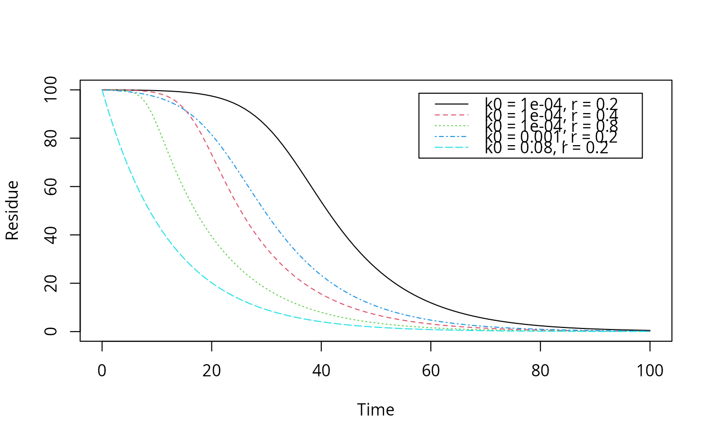
# Reproduce the plot on page 57 of FOCUS (2014) plot(function(x) logistic.solution(x, 100, 0.08, 0.0001, 0.2), from = 0, to = 100, ylim = c(0, 100), xlab = "Time", ylab = "Residue")plot(function(x) logistic.solution(x, 100, 0.08, 0.0001, 0.4), from = 0, to = 100, add = TRUE, lty = 2, col = 2)plot(function(x) logistic.solution(x, 100, 0.08, 0.0001, 0.8), from = 0, to = 100, add = TRUE, lty = 3, col = 3)plot(function(x) logistic.solution(x, 100, 0.08, 0.001, 0.2), from = 0, to = 100, add = TRUE, lty = 4, col = 4)plot(function(x) logistic.solution(x, 100, 0.08, 0.08, 0.2), from = 0, to = 100, add = TRUE, lty = 5, col = 5)legend("topright", inset = 0.05, legend = paste0("k0 = ", c(0.0001, 0.0001, 0.0001, 0.001, 0.08), ", r = ", c(0.2, 0.4, 0.8, 0.2, 0.2)), lty = 1:5, col = 1:5)# Fit with synthetic data logistic <- mkinmod(parent = mkinsub("logistic")) sampling_times = c(0, 1, 3, 7, 14, 28, 60, 90, 120) parms_logistic <- c(kmax = 0.08, k0 = 0.0001, r = 0.2) d_logistic <- mkinpredict(logistic, parms_logistic, c(parent = 100), sampling_times) d_2_1 <- add_err(d_logistic, sdfunc = function(x) sigma_twocomp(x, 0.5, 0.07), n = 1, reps = 2, digits = 5, LOD = 0.1, seed = 123456)[[1]] m <- mkinfit("logistic", d_2_1, quiet = TRUE) plot_sep(m)#> Estimate se_notrans t value Pr(>t) Lower #> parent_0 1.057896e+02 1.9023449649 55.610120 3.768361e-16 1.016451e+02 #> kmax 6.398190e-02 0.0143201029 4.467978 3.841828e-04 3.929235e-02 #> k0 1.612775e-04 0.0005866813 0.274898 3.940351e-01 5.846685e-08 #> r 2.263946e-01 0.1718110773 1.317695 1.061044e-01 4.335843e-02 #> sigma 5.332935e+00 0.9145907310 5.830952 4.036926e-05 3.340213e+00 #> Upper #> parent_0 109.9341588 #> kmax 0.1041853 #> k0 0.4448750 #> r 1.1821121 #> sigma 7.3256566#> DT50 DT90 DT50_k0 DT50_kmax #> parent 36.86533 62.41511 4297.854 10.83349