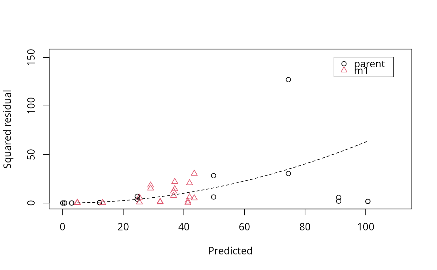
Function to plot squared residuals and the error model for an mkin object
mkinerrplot.RdThis function plots the squared residuals for the specified subset of the
observed variables from an mkinfit object. In addition, one or more
dashed line(s) show the fitted error model.
A combined plot of the fitted model and this error model plot can be
obtained with plot.mkinfit
using the argument show_errplot = TRUE.
mkinerrplot(object,
    obs_vars = names(object$mkinmod$map),
    xlim = c(0, 1.1 * max(object$data$predicted)),
    xlab = "Predicted", ylab = "Squared residual",
    maxy = "auto", legend= TRUE, lpos = "topright",
    col_obs = "auto", pch_obs = "auto",
    ...)
Arguments
| object | A fit represented in an |
|---|---|
| obs_vars | A character vector of names of the observed variables for which residuals should be plotted. Defaults to all observed variables in the model |
| xlim | plot range in x direction. |
| xlab | Label for the x axis. |
| ylab | Label for the y axis. |
| maxy | Maximum value of the residuals. This is used for the scaling of the y axis and defaults to "auto". |
| legend | Should a legend be plotted? |
| lpos | Where should the legend be placed? Default is "topright". Will be passed on to
|
| col_obs | Colors for the observed variables. |
| pch_obs | Symbols to be used for the observed variables. |
| … | further arguments passed to |
Value
Nothing is returned by this function, as it is called for its side effect, namely to produce a plot.
See also
mkinplot, for a way to plot the data and the fitted lines of the
mkinfit object.
Examples
#>#> Warning: Observations with value of zero were removed from the datamkinerrplot(fit)
