This functions sets up a nonlinear mixed effects model for an mmkin row object. An mmkin row object is essentially a list of mkinfit objects that have been obtained by fitting the same model to a list of datasets.
# S3 method for mmkin
nlme(
  model,
  data = sys.frame(sys.parent()),
  fixed,
  random = fixed,
  groups,
  start,
  correlation = NULL,
  weights = NULL,
  subset,
  method = c("ML", "REML"),
  na.action = na.fail,
  naPattern,
  control = list(),
  verbose = FALSE
)

# S3 method for nlme.mmkin
print(x, ...)

# S3 method for nlme.mmkin
update(object, ...)
Arguments
| model | An |
|---|---|
| data | Ignored, data are taken from the mmkin model |
| fixed | Ignored, all degradation parameters fitted in the mmkin model are used as fixed parameters |
| random | If not specified, all fixed effects are complemented with uncorrelated random effects |
| groups | See the documentation of nlme |
| start | If not specified, mean values of the fitted degradation parameters taken from the mmkin object are used |
| correlation | See the documentation of nlme |
| weights | passed to nlme |
| subset | passed to nlme |
| method | passed to nlme |
| na.action | passed to nlme |
| naPattern | passed to nlme |
| control | passed to nlme |
| verbose | passed to nlme |
| x | An nlme.mmkin object to print |
| ... | Update specifications passed to update.nlme |
| object | An nlme.mmkin object to update |
Value
Upon success, a fitted nlme.mmkin object, which is an nlme object with additional elements
See also
Examples
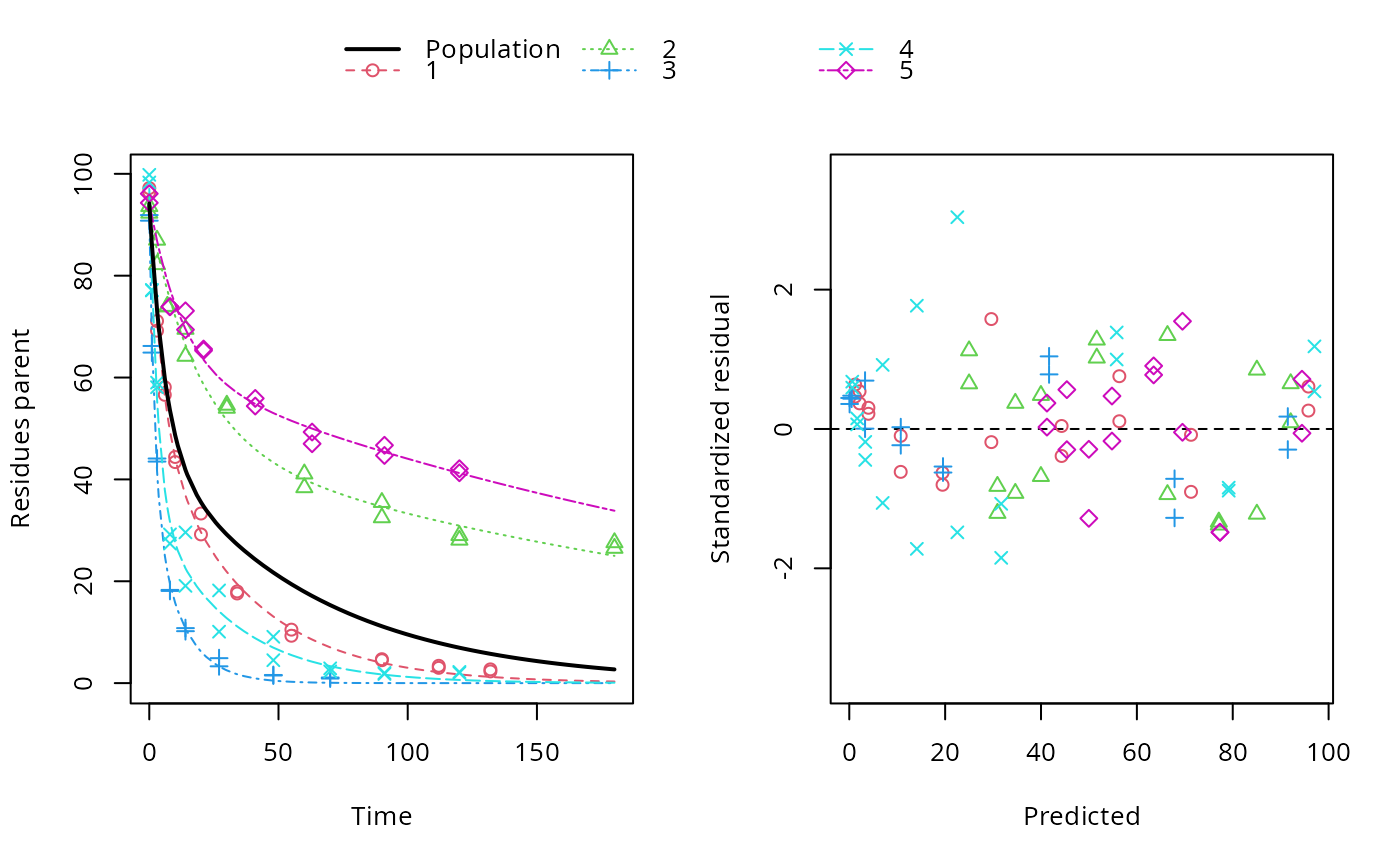
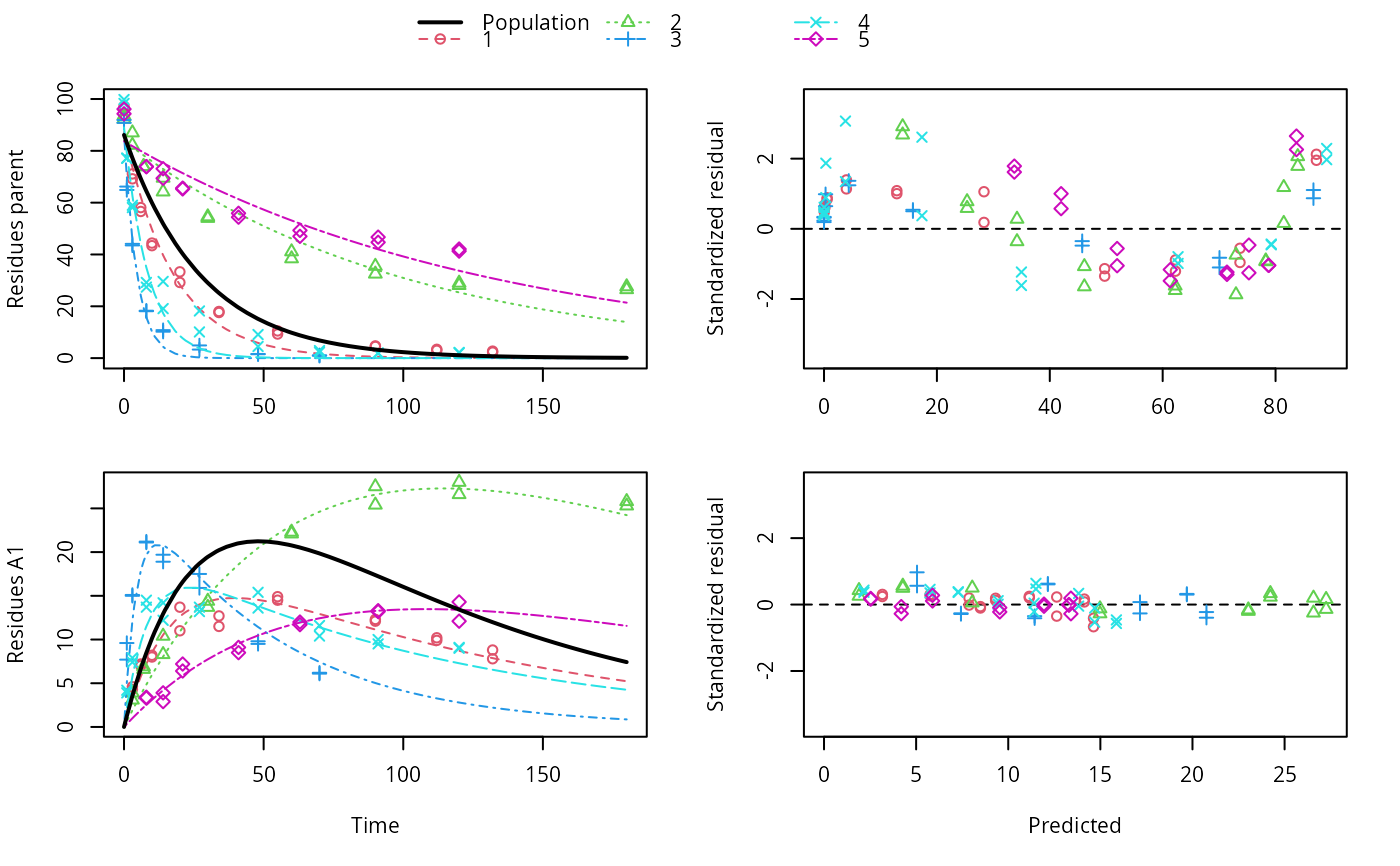
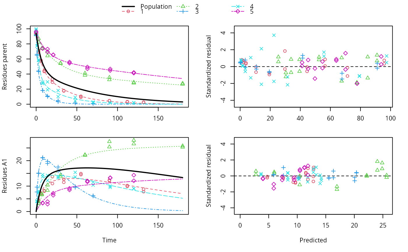
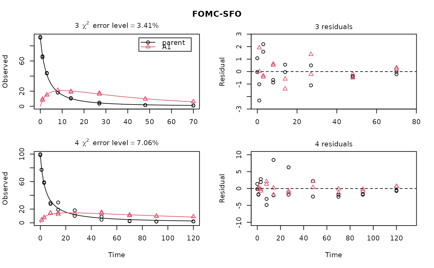
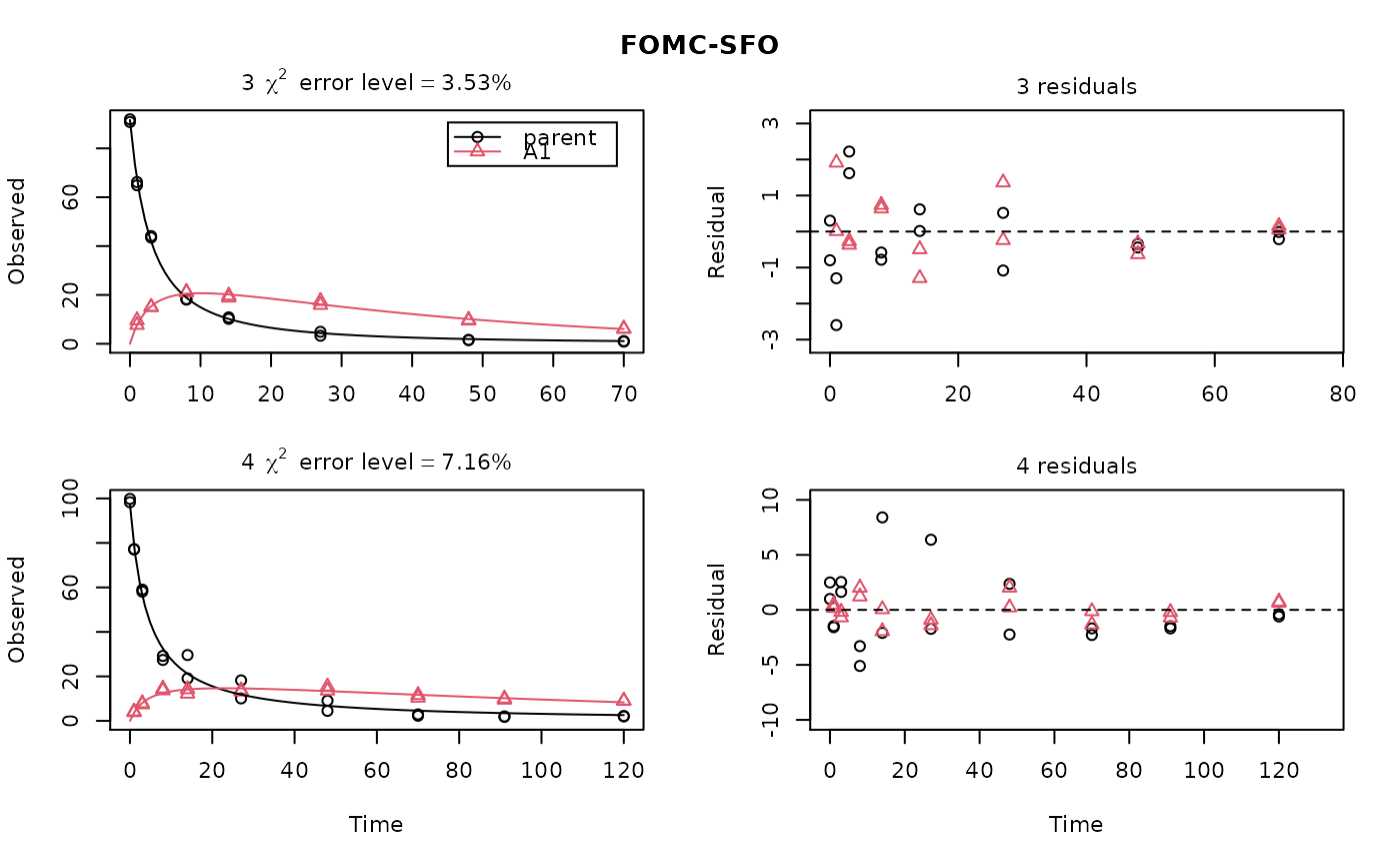
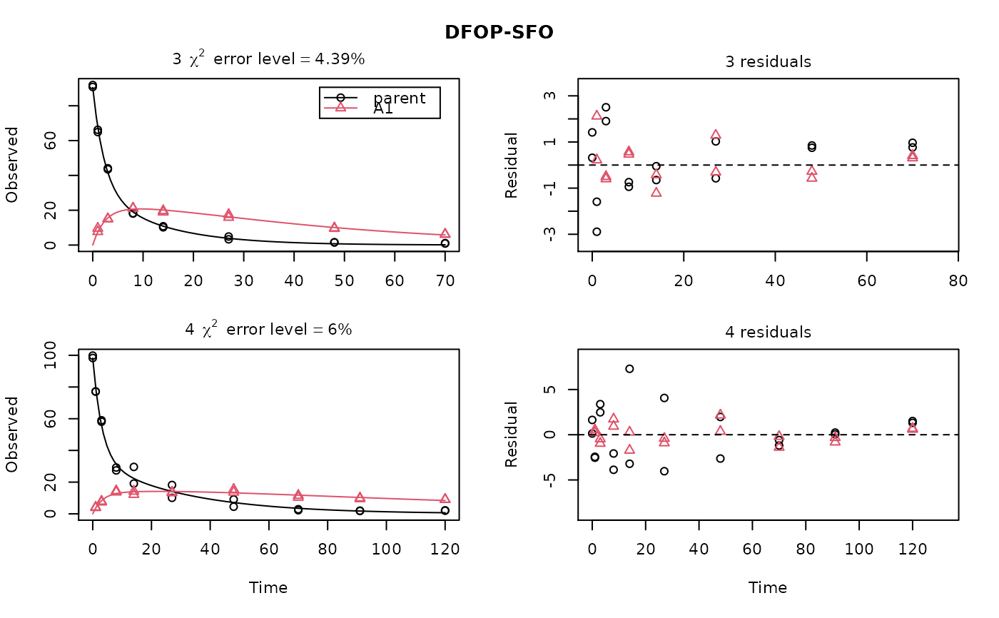
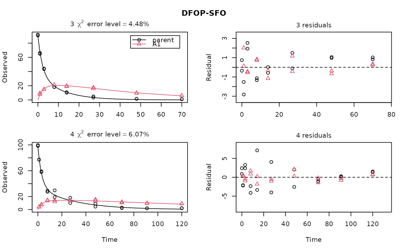
ds <- lapply(experimental_data_for_UBA_2019[6:10], function(x) subset(x$data[c("name", "time", "value")], name == "parent")) f <- mmkin("SFO", ds, quiet = TRUE, cores = 1)#> Warning: Shapiro-Wilk test for standardized residuals: p = 0.0195#> Warning: Shapiro-Wilk test for standardized residuals: p = 0.011#> $distimes #> DT50 DT90 #> parent 11.96183 39.73634 #>#> Nonlinear mixed-effects model fit by maximum likelihood #> Model: value ~ (mkin::get_deg_func())(name, time, parent_0, log_k_parent) #> Data: "Not shown" #> Log-likelihood: -307.5269 #> Fixed: list(parent_0 ~ 1, log_k_parent ~ 1) #> parent_0 log_k_parent #> 85.541149 -3.229596 #> #> Random effects: #> Formula: list(parent_0 ~ 1, log_k_parent ~ 1) #> Level: ds #> Structure: Diagonal #> parent_0 log_k_parent Residual #> StdDev: 1.30857 1.288591 6.304906 #> #> Number of Observations: 90 #> Number of Groups: 5#> $distimes #> DT50 DT90 #> parent 17.51545 58.18505 #># \dontrun{ f_nlme_2 <- nlme(f, start = c(parent_0 = 100, log_k_parent_sink = 0.1)) update(f_nlme_2, random = parent_0 ~ 1)#> Nonlinear mixed-effects model fit by maximum likelihood #> Model: value ~ (mkin::get_deg_func())(name, time, parent_0, log_k_parent) #> Data: "Not shown" #> Log-likelihood: -404.3729 #> Fixed: list(parent_0 ~ 1, log_k_parent ~ 1) #> parent_0 log_k_parent #> 75.933480 -3.555983 #> #> Random effects: #> Formula: parent_0 ~ 1 | ds #> parent_0 Residual #> StdDev: 0.002416792 21.63027 #> #> Number of Observations: 90 #> Number of Groups: 5# Test on some real data ds_2 <- lapply(experimental_data_for_UBA_2019[6:10], function(x) x$data[c("name", "time", "value")]) m_sfo_sfo <- mkinmod(parent = mkinsub("SFO", "A1"), A1 = mkinsub("SFO"), use_of_ff = "min", quiet = TRUE) m_sfo_sfo_ff <- mkinmod(parent = mkinsub("SFO", "A1"), A1 = mkinsub("SFO"), use_of_ff = "max", quiet = TRUE) m_fomc_sfo <- mkinmod(parent = mkinsub("FOMC", "A1"), A1 = mkinsub("SFO"), quiet = TRUE) m_dfop_sfo <- mkinmod(parent = mkinsub("DFOP", "A1"), A1 = mkinsub("SFO"), quiet = TRUE) f_2 <- mmkin(list("SFO-SFO" = m_sfo_sfo, "SFO-SFO-ff" = m_sfo_sfo_ff, "FOMC-SFO" = m_fomc_sfo, "DFOP-SFO" = m_dfop_sfo), ds_2, quiet = TRUE) plot(f_2["SFO-SFO", 3:4]) # Separate fits for datasets 3 and 4f_nlme_sfo_sfo <- nlme(f_2["SFO-SFO", ]) # plot(f_nlme_sfo_sfo) # not feasible with pkgdown figures plot(f_nlme_sfo_sfo, 3:4) # Global mixed model: Fits for datasets 3 and 4# With formation fractions f_nlme_sfo_sfo_ff <- nlme(f_2["SFO-SFO-ff", ]) plot(f_nlme_sfo_sfo_ff, 3:4) # chi2 different due to different df attribution# For more parameters, we need to increase pnlsMaxIter and the tolerance # to get convergence f_nlme_fomc_sfo <- nlme(f_2["FOMC-SFO", ], control = list(pnlsMaxIter = 100, tolerance = 1e-4), verbose = TRUE)#> #> **Iteration 1 #> LME step: Loglik: -394.1603, nlminb iterations: 3 #> reStruct parameters: #> ds1 ds2 ds3 ds4 ds5 #> -0.2079793 0.8563830 1.7454105 1.0917354 1.2756825 #> Beginning PNLS step: .. completed fit_nlme() step. #> PNLS step: RSS = 643.8803 #> fixed effects: 94.17379 -5.473193 -0.6970236 -0.2025091 2.103883 #> iterations: 100 #> Convergence crit. (must all become <= tolerance = 0.0001): #> fixed reStruct #> 0.7960134 0.1447728 #> #> **Iteration 2 #> LME step: Loglik: -396.3824, nlminb iterations: 7 #> reStruct parameters: #> ds1 ds2 ds3 ds4 ds5 #> -1.712404e-01 -2.432655e-05 1.842120e+00 1.073975e+00 1.322925e+00 #> Beginning PNLS step: .. completed fit_nlme() step. #> PNLS step: RSS = 643.8035 #> fixed effects: 94.17385 -5.473487 -0.6970404 -0.2025137 2.103871 #> iterations: 100 #> Convergence crit. (must all become <= tolerance = 0.0001): #> fixed reStruct #> 5.382757e-05 1.236667e-03 #> #> **Iteration 3 #> LME step: Loglik: -396.3825, nlminb iterations: 7 #> reStruct parameters: #> ds1 ds2 ds3 ds4 ds5 #> -0.1712499044 -0.0001499831 1.8420971364 1.0739799123 1.3229167796 #> Beginning PNLS step: .. completed fit_nlme() step. #> PNLS step: RSS = 643.7948 #> fixed effects: 94.17386 -5.473521 -0.6970422 -0.2025144 2.10387 #> iterations: 100 #> Convergence crit. (must all become <= tolerance = 0.0001): #> fixed reStruct #> 6.072817e-06 1.400857e-04 #> #> **Iteration 4 #> LME step: Loglik: -396.3825, nlminb iterations: 7 #> reStruct parameters: #> ds1 ds2 ds3 ds4 ds5 #> -0.1712529502 -0.0001641277 1.8420957542 1.0739797181 1.3229173076 #> Beginning PNLS step: .. completed fit_nlme() step. #> PNLS step: RSS = 643.7936 #> fixed effects: 94.17386 -5.473526 -0.6970426 -0.2025146 2.103869 #> iterations: 100 #> Convergence crit. (must all become <= tolerance = 0.0001): #> fixed reStruct #> 1.027451e-06 2.275704e-05f_nlme_dfop_sfo <- nlme(f_2["DFOP-SFO", ], control = list(pnlsMaxIter = 120, tolerance = 5e-4), verbose = TRUE)#> #> **Iteration 1 #> LME step: Loglik: -404.9582, nlminb iterations: 1 #> reStruct parameters: #> ds1 ds2 ds3 ds4 ds5 ds6 #> -0.4114355 0.9798697 1.6990037 0.7293315 0.3354323 1.7113046 #> Beginning PNLS step: .. completed fit_nlme() step. #> PNLS step: RSS = 630.3644 #> fixed effects: 93.82269 -5.455991 -0.6788957 -1.862196 -4.199671 0.05532828 #> iterations: 120 #> Convergence crit. (must all become <= tolerance = 0.0005): #> fixed reStruct #> 0.7885368 0.5822683 #> #> **Iteration 2 #> LME step: Loglik: -407.7755, nlminb iterations: 11 #> reStruct parameters: #> ds1 ds2 ds3 ds4 ds5 ds6 #> -0.371224133 0.003056179 1.789939402 0.724671158 0.301602977 1.754200729 #> Beginning PNLS step: .. completed fit_nlme() step. #> PNLS step: RSS = 630.3633 #> fixed effects: 93.82269 -5.455992 -0.6788958 -1.862196 -4.199671 0.05532831 #> iterations: 120 #> Convergence crit. (must all become <= tolerance = 0.0005): #> fixed reStruct #> 4.789774e-07 2.200661e-05#> Model df AIC BIC logLik Test L.Ratio p-value #> f_nlme_dfop_sfo 1 13 843.8547 884.6201 -408.9273 #> f_nlme_fomc_sfo 2 11 818.5149 853.0087 -398.2575 1 vs 2 21.33975 <.0001 #> f_nlme_sfo_sfo 3 9 1085.1821 1113.4043 -533.5910 2 vs 3 270.66716 <.0001#> Model df AIC BIC logLik Test L.Ratio p-value #> f_nlme_dfop_sfo 1 13 843.8547 884.6201 -408.9273 #> f_nlme_sfo_sfo 2 9 1085.1821 1113.4043 -533.5910 1 vs 2 249.3274 <.0001#> $ff #> parent_sink parent_A1 A1_sink #> 0.5912432 0.4087568 1.0000000 #> #> $distimes #> DT50 DT90 #> parent 19.13518 63.5657 #> A1 66.02155 219.3189 #>#> $ff #> parent_A1 parent_sink #> 0.2768574 0.7231426 #> #> $distimes #> DT50 DT90 DT50back DT50_k1 DT50_k2 #> parent 11.07091 104.6320 31.49738 4.462384 46.20825 #> A1 162.30536 539.1667 NA NA NA #># }