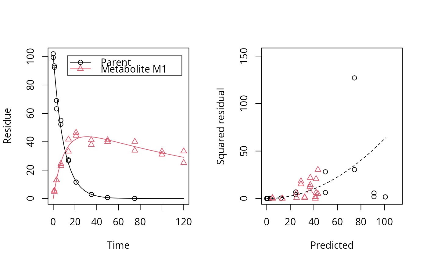
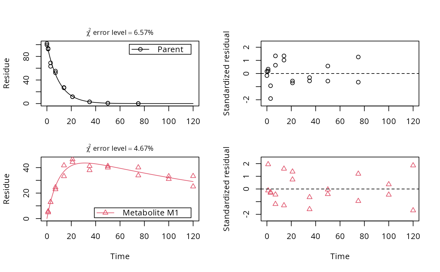
Solves the differential equations with the optimised and fixed parameters from a previous successful call to mkinfit and plots the observed data together with the solution of the fitted model.

# S3 method for mkinfit
plot(x, fit = x,
  obs_vars = names(fit$mkinmod$map),
  xlab = "Time", ylab = "Observed", 
  xlim = range(fit$data$time),
  ylim = "default",
  col_obs = 1:length(obs_vars), pch_obs = col_obs, 
  lty_obs = rep(1, length(obs_vars)),
  add = FALSE, legend = !add,
  show_residuals = FALSE, maxabs = "auto",
  sep_obs = FALSE, rel.height.middle = 0.9,
  lpos = "topright", inset = c(0.05, 0.05), 
  show_errmin = FALSE, errmin_digits = 3, …)
plot_sep(fit, sep_obs = TRUE,  show_residuals = TRUE, show_errmin = TRUE, …)

Arguments

x

Alias for fit introduced for compatibility with the generic S3 method.

fit

An object of class mkinfit.

obs_vars

A character vector of names of the observed variables for which the data and the model should be plotted. Defauls to all observed variables in the model.

xlab

Label for the x axis.

ylab

Label for the y axis.

xlim

Plot range in x direction.

ylim

Plot range in y direction.

col_obs

Colors used for plotting the observed data and the corresponding model prediction lines.

pch_obs

Symbols to be used for plotting the data.

lty_obs

Line types to be used for the model predictions.

add

Should the plot be added to an existing plot?

legend

Should a legend be added to the plot?

show_residuals

Should residuals be shown? If only one plot of the fits is shown, the residual plot is in the lower third of the plot? Otherwise, i.e. if "sep_obs" is given, the residual plots will be located to the right of the plots of the fitted curves.

maxabs

Maximum absolute value of the residuals. This is used for the scaling of the y axis and defaults to "auto".

sep_obs

Should the observed variables be shown in separate subplots? If yes, residual plots requested by "show_residuals" will be shown next to, not below the plot of the fits.

rel.height.middle

The relative height of the middle plot, if more than two rows of plots are shown.

lpos

Position(s) of the legend(s). Passed to legend as the first argument. If not length one, this should be of the same length as the obs_var argument.

inset

Passed to legend if applicable.

show_errmin

Should the FOCUS chi2 error value be shown in the upper margin of the plot?

errmin_digits

The number of significant digits for rounding the FOCUS chi2 error percentage.

…

Further arguments passed to plot.

Value

The function is called for its side effect.

Examples

# One parent compound, one metabolite, both single first order, path from
# parent to sink included, use Levenberg-Marquardt for speed
SFO_SFO <- mkinmod(parent = mkinsub("SFO", "m1", full = "Parent"),
                   m1 = mkinsub("SFO", full = "Metabolite M1" ))
Successfully compiled differential equation model from auto-generated C code.
fit <- mkinfit(SFO_SFO, FOCUS_2006_D, quiet = TRUE, method.modFit = "Marq")
plot(fit)
plot(fit, show_residuals = TRUE)

# Show the observed variables separately
plot(fit, sep_obs = TRUE, lpos = c("topright", "bottomright"))

# Show the observed variables separately, with residuals
plot(fit, sep_obs = TRUE, show_residuals = TRUE, lpos = c("topright", "bottomright"),
     show_errmin = TRUE)

# The same can be obtained with less typing, using the convenience function plot_sep
plot_sep(fit, lpos = c("topright", "bottomright"))