Plot the observed data and the fitted model of an mkinfit object

Solves the differential equations with the optimised and fixed parameters from a previous successful call to mkinfit and plots the observed data together with the solution of the fitted model.

Usage

# S3 method for mkinfit
plot(
  x,
  fit = x,
  obs_vars = names(fit$mkinmod$map),
  xlab = "Time",
  ylab = "Residue",
  xlim = range(fit$data$time),
  ylim = "default",
  col_obs = 1:length(obs_vars),
  pch_obs = col_obs,
  lty_obs = rep(1, length(obs_vars)),
  add = FALSE,
  legend = !add,
  show_residuals = FALSE,
  show_errplot = FALSE,
  maxabs = "auto",
  sep_obs = FALSE,
  rel.height.middle = 0.9,
  row_layout = FALSE,
  lpos = "topright",
  inset = c(0.05, 0.05),
  show_errmin = FALSE,
  errmin_digits = 3,
  frame = TRUE,
  ...
)

plot_sep(
  fit,
  show_errmin = TRUE,
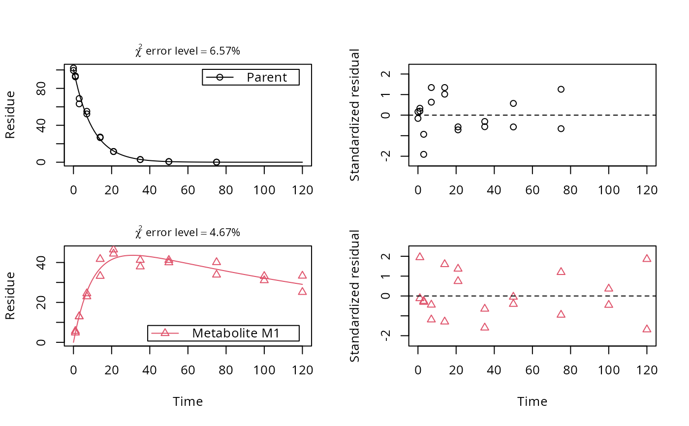
  show_residuals = ifelse(identical(fit$err_mod, "const"), TRUE, "standardized"),
  ...
)

plot_res(
  fit,
  sep_obs = FALSE,
  show_errmin = sep_obs,
  standardized = ifelse(identical(fit$err_mod, "const"), FALSE, TRUE),
  ...
)

plot_err(fit, sep_obs = FALSE, show_errmin = sep_obs, ...)

Arguments

x: Alias for fit introduced for compatibility with the generic S3 method.
fit: An object of class mkinfit.
obs_vars: A character vector of names of the observed variables for which the data and the model should be plotted. Defauls to all observed variables in the model.
xlab: Label for the x axis.
ylab: Label for the y axis.
xlim: Plot range in x direction.
ylim: Plot range in y direction. If given as a list, plot ranges for the different plot rows can be given for row layout.
col_obs: Colors used for plotting the observed data and the corresponding model prediction lines.
pch_obs: Symbols to be used for plotting the data.
lty_obs: Line types to be used for the model predictions.
add: Should the plot be added to an existing plot?
legend: Should a legend be added to the plot?
show_residuals: Should residuals be shown? If only one plot of the fits is shown, the residual plot is in the lower third of the plot. Otherwise, i.e. if "sep_obs" is given, the residual plots will be located to the right of the plots of the fitted curves. If this is set to 'standardized', a plot of the residuals divided by the standard deviation given by the fitted error model will be shown.
show_errplot: Should squared residuals and the error model be shown? If only one plot of the fits is shown, this plot is in the lower third of the plot. Otherwise, i.e. if "sep_obs" is given, the residual plots will be located to the right of the plots of the fitted curves.
maxabs: Maximum absolute value of the residuals. This is used for the scaling of the y axis and defaults to "auto".
sep_obs: Should the observed variables be shown in separate subplots? If yes, residual plots requested by "show_residuals" will be shown next to, not below the plot of the fits.
rel.height.middle: The relative height of the middle plot, if more than two rows of plots are shown.
row_layout: Should we use a row layout where the residual plot or the error model plot is shown to the right?
lpos: Position(s) of the legend(s). Passed to legend as the first argument. If not length one, this should be of the same length as the obs_var argument.
inset: Passed to legend if applicable.
show_errmin: Should the FOCUS chi2 error value be shown in the upper margin of the plot?
errmin_digits: The number of significant digits for rounding the FOCUS chi2 error percentage.
frame: Should a frame be drawn around the plots?
...: Further arguments passed to plot.
standardized: When calling 'plot_res', should the residuals be standardized in the residual plot?

Value

The function is called for its side effect.

Details

If the current plot device is a tikz device, then latex is being used for the formatting of the chi2 error level, if show_errmin = TRUE.

Author

Johannes Ranke

Examples


# One parent compound, one metabolite, both single first order, path from
# parent to sink included
# \dontrun{
SFO_SFO <- mkinmod(parent = mkinsub("SFO", "m1", full = "Parent"),
                   m1 = mkinsub("SFO", full = "Metabolite M1" ))
#> Temporary DLL for differentials generated and loaded
fit <- mkinfit(SFO_SFO, FOCUS_2006_D, quiet = TRUE)
#> Warning: Observations with value of zero were removed from the data
fit <- mkinfit(SFO_SFO, FOCUS_2006_D, quiet = TRUE, error_model = "tc")
#> Warning: Observations with value of zero were removed from the data
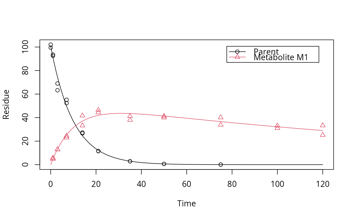
plot(fit)

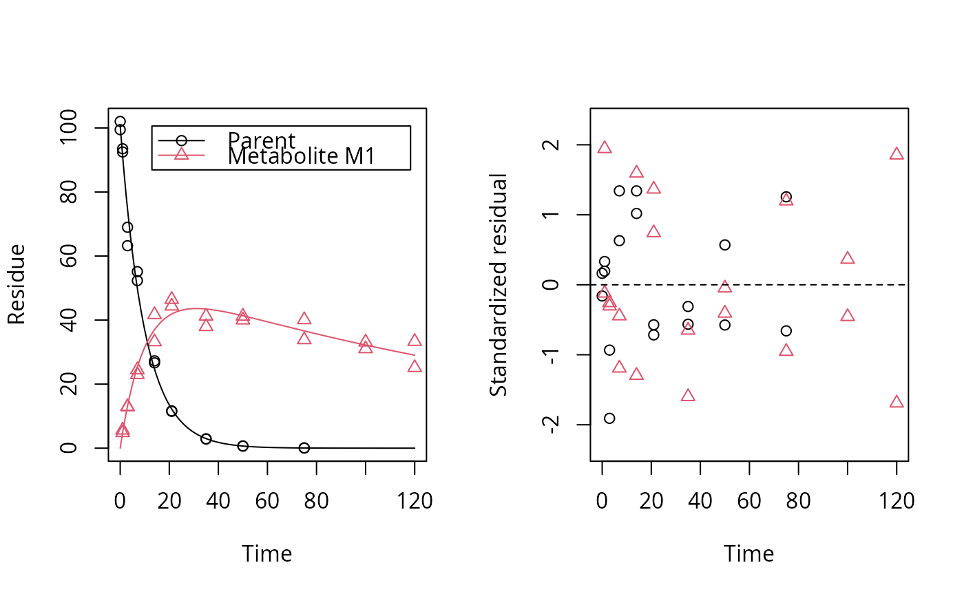
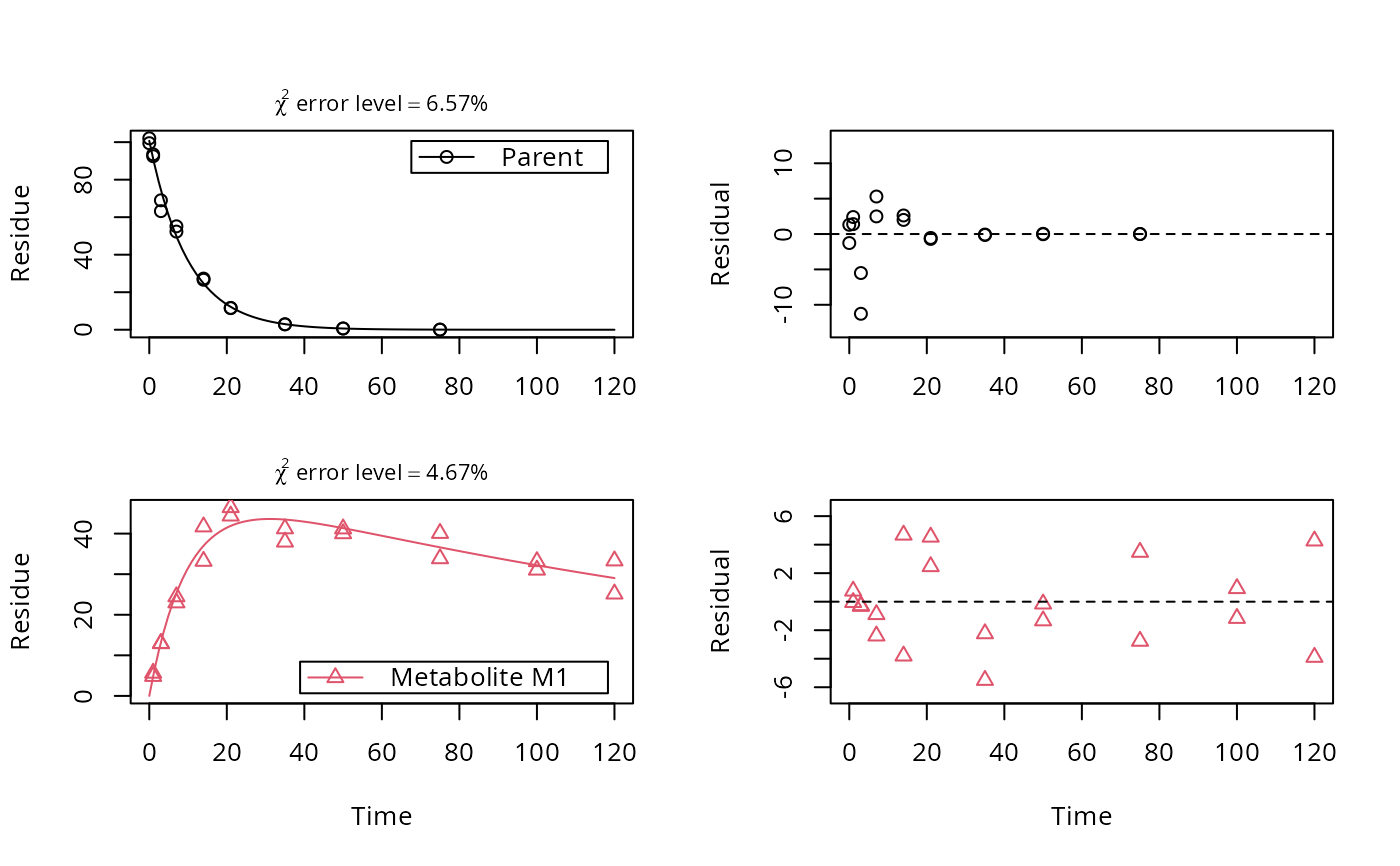
plot_res(fit)

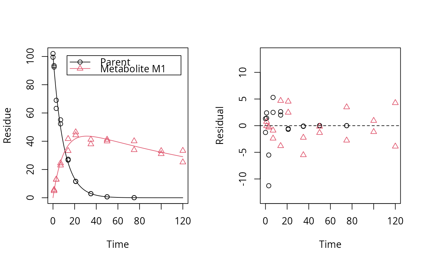
plot_res(fit, standardized = FALSE)

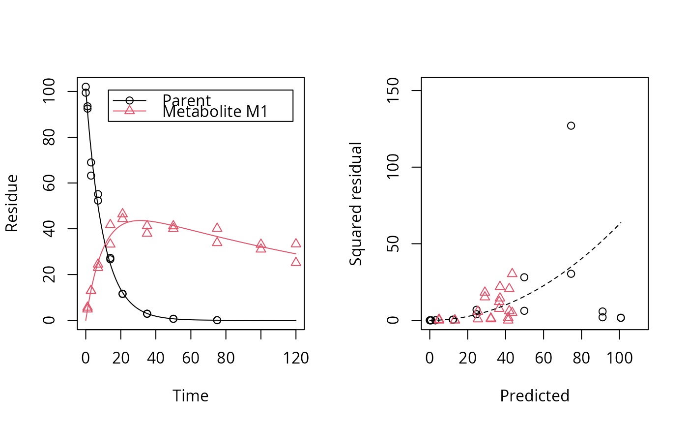
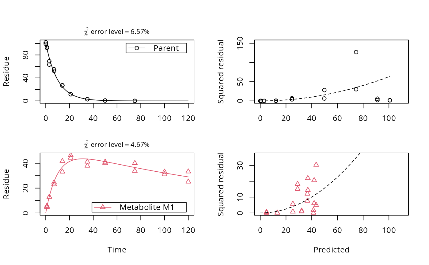
plot_err(fit)


# Show the observed variables separately, with residuals
plot(fit, sep_obs = TRUE, show_residuals = TRUE, lpos = c("topright", "bottomright"),
     show_errmin = TRUE)


# The same can be obtained with less typing, using the convenience function plot_sep
plot_sep(fit, lpos = c("topright", "bottomright"))


# Show the observed variables separately, with the error model
plot(fit, sep_obs = TRUE, show_errplot = TRUE, lpos = c("topright", "bottomright"),
     show_errmin = TRUE)

# }