Three experimental datasets from two water sediment systems and one soil
test_data_from_UBA_2014.RdThe datasets were used for the comparative validation of several kinetic evaluation software packages (Ranke, 2014).
test_data_from_UBA_2014
Format
A list containing three datasets as an R6 class defined by mkinds.
Each dataset has, among others, the following components
titleThe name of the dataset, e.g.
UBA_2014_WS_riverdataA data frame with the data in the form expected by
mkinfit
Source
Ranke (2014) Prüfung und Validierung von Modellierungssoftware als Alternative zu ModelMaker 4.0, Umweltbundesamt Projektnummer 27452
Examples
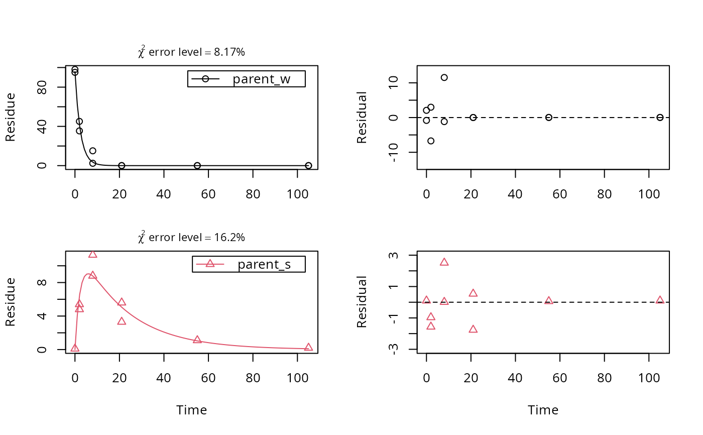
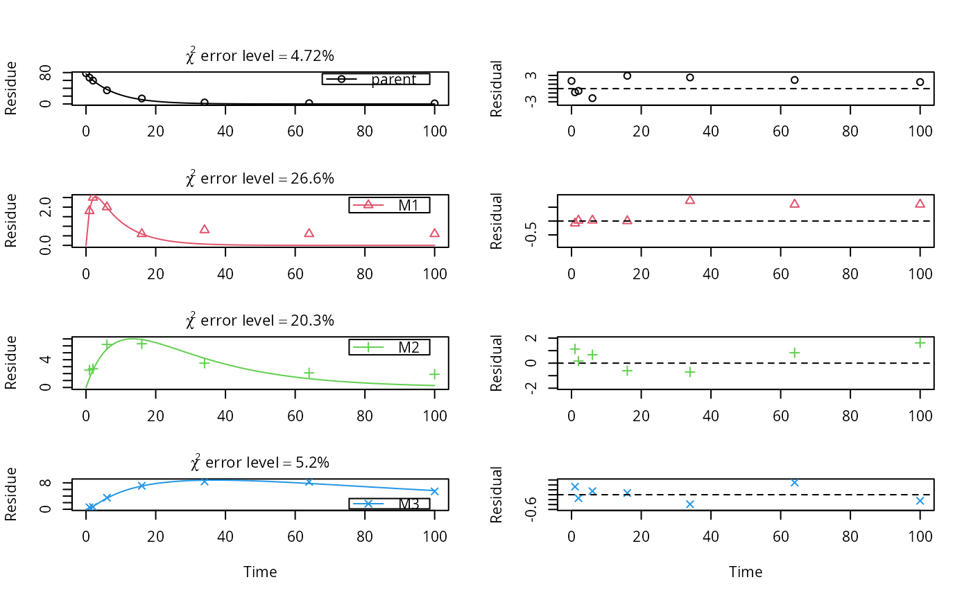
# This is a level P-II evaluation of the dataset according to the FOCUS kinetics # guidance. Due to the strong correlation of the parameter estimates, the # covariance matrix is not returned. Note that level P-II evaluations are # generally considered deprecated due to the frequent occurrence of such # large parameter correlations, among other reasons (e.g. the adequacy of the # model). m_ws <- mkinmod(parent_w = mkinsub("SFO", "parent_s"), parent_s = mkinsub("SFO", "parent_w"))#>#> Estimate se_notrans t value Pr(>t) Lower #> parent_w_0 9.598567e+01 2.33959800 4.102657e+01 9.568967e-19 NA #> k_parent_w_sink 3.603743e-01 0.03497750 1.030303e+01 4.989002e-09 NA #> k_parent_w_parent_s 6.031371e-02 0.01746024 3.454346e+00 1.514723e-03 NA #> k_parent_s_sink 5.108539e-11 0.10382001 4.920572e-10 5.000000e-01 NA #> k_parent_s_parent_w 7.419672e-02 0.11338240 6.543936e-01 2.608069e-01 NA #> Upper #> parent_w_0 NA #> k_parent_w_sink NA #> k_parent_w_parent_s NA #> k_parent_s_sink NA #> k_parent_s_parent_w NAmkinerrmin(f_river)#> err.min n.optim df #> All data 0.09246946 5 6 #> parent_w 0.06377096 3 3 #> parent_s 0.20882324 2 3# This is the evaluation used for the validation of software packages # in the expertise from 2014 m_soil <- mkinmod(parent = mkinsub("SFO", c("M1", "M2")), M1 = mkinsub("SFO", "M3"), M2 = mkinsub("SFO", "M3"), M3 = mkinsub("SFO"), use_of_ff = "max")#>f_soil <- mkinfit(m_soil, test_data_from_UBA_2014[[3]]$data, quiet = TRUE) plot_sep(f_soil, lpos = c("topright", "topright", "topright", "bottomright"))#> Estimate se_notrans t value Pr(>t) Lower #> parent_0 76.55425584 0.943443794 81.1434198 4.422336e-30 74.602593773 #> k_parent 0.12081956 0.004815515 25.0896457 1.639665e-18 0.111257517 #> k_M1 0.84258651 0.930121548 0.9058886 1.871938e-01 0.085876516 #> k_M2 0.04210878 0.013729902 3.0669396 2.729137e-03 0.021450630 #> k_M3 0.01122919 0.008044865 1.3958206 8.804912e-02 0.002550984 #> f_parent_to_M1 0.32240199 0.278620579 1.1571363 1.295467e-01 NA #> f_parent_to_M2 0.16099854 0.030548888 5.2701931 1.196190e-05 NA #> f_M1_to_M3 0.27921500 0.314732842 0.8871492 1.920908e-01 0.015016983 #> f_M2_to_M3 0.55641333 0.650246995 0.8556954 2.004966e-01 0.005360555 #> Upper #> parent_0 78.50591790 #> k_parent 0.13120341 #> k_M1 8.26712661 #> k_M2 0.08266188 #> k_M3 0.04942981 #> f_parent_to_M1 NA #> f_parent_to_M2 NA #> f_M1_to_M3 0.90777163 #> f_M2_to_M3 0.99658633mkinerrmin(f_soil)#> err.min n.optim df #> All data 0.09649963 9 20 #> parent 0.04721283 2 6 #> M1 0.26551209 2 5 #> M2 0.20327575 2 5 #> M3 0.05196549 3 4